
2d Foil Optimization
Updated November 14, 2023
Preliminary considerations
Optimizer
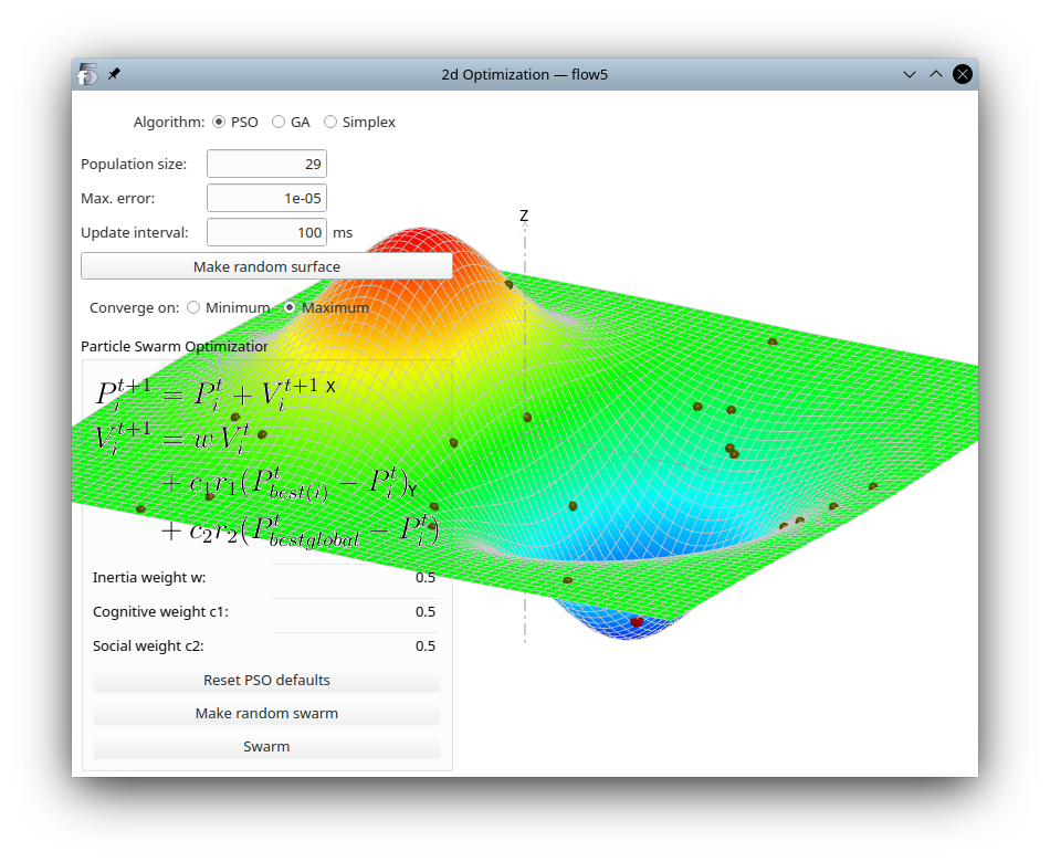
The 2d foil optimization module uses the Multi-Objective Particle Swarm Optimization (MOPSO) algorithm. The principle of the algorithm is described here.
A 2d visual demonstrator of the Particle Swarm Optimization and of the Genetic Algorithm can be accessed in xflr5 using the keyboard shortcut Ctrl+0 and F11.
This demonstrator can be used to test the influence of the algorithm's key parameters.
In the present case, a particle is a foil defined by the seed foil and a set of design variables.
The particle's fitness is the subset of the objective values {Cl, Cd, Cl/Cd, max.(Cpmin), Cm, Cm0} at the specified operating point.
Geometry modification
The principle is to start with a seed foil, and to make incremental modifications to its geometry so that is satisfies certain requirements.
The modifications are made by adding bumps in the shape of Hicks-Henne functions to the top and bottom surfaces. These bumps can be positive or negative, i.e. they will tend to move the surface outwards or inwards.
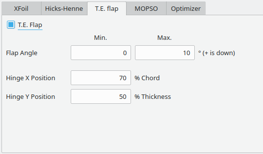
The trailing edge flap angle is an additional optional design variable.

Design objectives
The goal is to optimize any subset of the following four objectives at a specified operating point:
- lift coefficient
- drag coefficient
- glide ratio
- minimum pressure coefficient
XFoil convergence
An additional difficulty in the present case is that XFoil's convergence is not guaranteed, especially in the case of foils modified by bump functions. Those tend to generate wobbly surfaces which hinder XFoil's convergence.
An unconverged XFoil run for a given particle will not stop the optimizer as the particle is just ignored when building the Pareto front. However if too many particles are unconverged and ignored, the effect will be to reduce the effectiveness of the optimizer.
Step by step
Seed foil
The seed foil is the one currently selected in the Direct Analysis Module (Ctrl+5). To facilitate the convergence of the optimizer, it is good practice to use a seed airfoil with properties close to those that are targeted. Optimization can proceed by requesting incremental improvements.
Select the airfoil and make sure that the paneling is sufficiently fine for XFoil's convergence, but not too large to limit execution times.
Once selected, the optimizer is launched via the menu option "Design/Optimize" or by the shortcut F12.
Operating point
As of xflr5 v6.60, the optimizer only supports optimization for one operating point at a time. However the operating point can be changed at any time in the optimization process.
Design variables
The design variables for the optimization are the bump functions added to the top and bottom surfaces, and optionally the angle of the trailing edge flap.
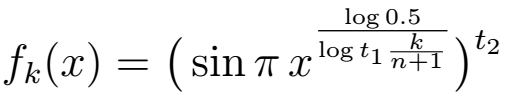
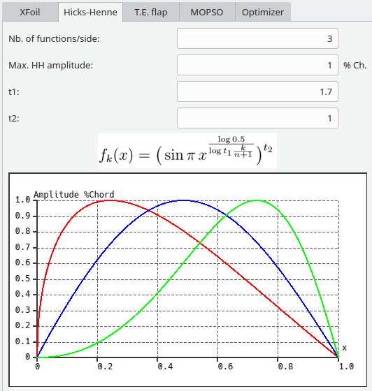
Hicks-Henne Bump functions
The functions are controlled by four values: the number of bump functions, their amplitude as a percentage of the chord length, and parameters t1 and t2. Adjust these settings so that:
- The bump functions are smooth and overlap; this is to increase the convergence probability of XFoil.
- The bump functions cover at least the part of the foil which needs to be optimized; ideally this should be the whole surface of the foil to give maximum freedom to the optimizer.
- The amplitude of the bump functions is low, typically 1% of the chord length. Here too high amplitudes will increase the wobbliness of the foil's surface.
Each bump function creates two design variables, one for the top surface and one for the bottom surface. Increasing the number of bump functions extends the design space, which may in turn increase the chances of finding a solution to the optimization problem. On the other hand it will also increase the surface's wobbliness.
Trailing Edge (TE) flap
Optionally the TE flap angle can be activated as an additional design variable.
If activated, the flap parameters will override those of the seed foil.
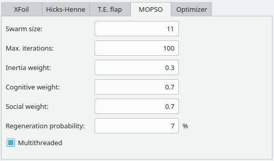
MOPSO settings
The signification and use of the parameters is explained here.
Swarm size
Experimentation so far has shown that a swarm size slightly greater than the number of design variables is sufficient to achieve optimization success in most cases.
For instance if 3 bump functions/side have been selected and the TE flap is activated, the number of design variables is 2x3+1=7, and the swarm population should typically be between 7 to 15.
Regeneration probability
It can occur that the swarm converges and gets stuck on a local optimum. To avoid this from occurring or from lasting too long, each particle has a probability to be teleported to a random location at each iteration. This probability should typically be in the range of 5% to 25%.
Other settings
The other parameters are intended for advanced users and should be left to their default values for the first runs.
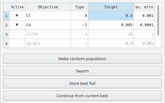
Design objectives
The four design objectives which are available are the lift and drag coefficient, the glide ratio and the minimum value of the pressure coefficients.
At least one objective needs to be active, and any subset of the four objectives can be activated. There is however redundancy in the first three objectives. It is therefore inadvisable to select all three of them at the same time since this may lead to conflicts and to an unsolvable problem.
Typically, the objective is to maximize the lift or glide ratio, to minimize the drag, and to maximize the minimum pressure coefficient.
It is also possible instead to target a specified value. The behaviour is defined by the "Type" in the third column. Set the value to 1 if the objective is to MAXIMIZE, to 0 if it is to EQUALIZE, and to -1 to MINIMIZE.
If the objective is to MAXIMIZE (resp. MINIMIZE) any value greater than (resp. lower than) the target is considered a success.
If the objective is to EQUALIZE, the success is achieved once the objective is within the error margin defined in the last column. This error is ignored in the MAXIMIZE and MINIMIZE cases.
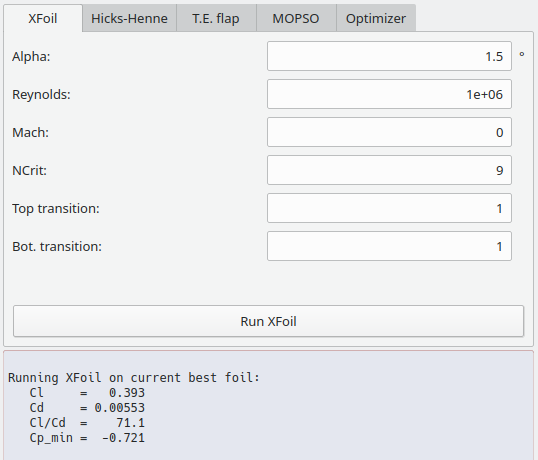
To identify reasonable values for the design objectives, it is possible to go to the "XFoil" tab and click "Run XFoil". The values of the objectives for the seed foil will be output in the bottom panel.
Execution
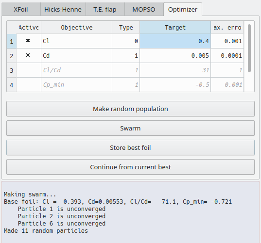
Random population
The first step is to make a random population of particles. At this first step, it should be paid attention to the convergence success of XFoil. If for instance more than a third of the particles didn't converge, an adjustment of the design variables should be considered before proceeding further.
Swarming
The progress of the optimization is shown in the output pane and in the graph objectives.Attention should be paid to the convergence success of XFoil.
If the optimization is unsuccessful, swarming can be resumed using the latest particle swarm by simply clicking the swarm button again, or a new swarm can be generated.
The input parameters can be modified when the task is not running. When resumed, the optimizer will start with the last swarm and the new parameters for input.
However, a modification of the number of design variables or of the number of objectives will change the corresponding dimensions of the design space, and will force a rebuild of the swarm.
Whether the optimization is successful or not, the "Store best foil" can be used to add the swarm's "best" foil to the internal database of foil's. The "best" foil is arbitrarily chosen to be the first listed in the Pareto front.
Clicking the button "Continue from current best" will replace the seed foil by the current best, which is added to the internal array of foils.
The XFoil analysis settings can be changed to optimize for a different operating point. This will likely deteriorate the optimization for any previous operating point.
Note: If the surface of the optimized foil is too wobbly, exit the optimizer and use the splines in the Direct Foil Design module to rebuild a smooth airfoil.
Back to top