Multi-Objective Particle Swarm Optimization

Contents

• Theoretical background
  • Single-objective Particle Swarm Optimization
  • Multi-Objective Particle Swarm Optimization
  • PSO 2d demo and proof of concept
  • Application to airplane optimizations
• Step by step
• Start configuration
• Interface
• Objectives
• Variables
• MOPSO parameters
• Analysis
• Optimization run
• Results

Theoretical background

flow5 v7.07 introduces a new module for the optimization of planes using the Multi-Objective Particle Swarm Optimization (MOPSO) algorithm. This algorithm and its many variants are well documented elsewhere, so that only the main features important to the correct use of the algorithm are mentioned here.

Single-objective Particle Swarm Optimization (PSO)

In its original and simplest form, the algorithm performs the optimization of a function towards a single objective and is designated by the acronym PSO. The general principle is to perform the optimization process in a manner similar to the one by which a swarm of birds or insects converges towards its target.

PSO vs. Genetic Algorithm

An alternative to the PSO is the Genetic Algorithm (GA). Preliminary tests performed in flow5 have shown so far that the GA does not converge as fast as the PSO, and tends to get stuck on local optimums. This is not a general conclusion however and is likely due to the specificities of the algorithm's implementation in flow5.

Given its apparent robustness, its simplicity and its versatility, the PSO has been selected as the algorithm to use in flow5.

Particle definition

Each of the swarm's particle is fully determined by its position in the space of variables, and by its velocity in this same space.
The space of variables in which the optimization is to be performed is determined by the user. It can be for instance the plane's CoG position, the main wing's aspect ratio and the elevator's tilt angle, in which case the design space has dimension 3.

The particle's position is used to evaluate its fitness vs. each objective, i.e. the value of the objective function at the particle's location, and the error or distance to the objectives.

Particle movement

All particles are moved simultaneously at each iteration.

The change of velocity of each particle follows loosely the laws of mechanic, with randomizing factors added in to increase the swarm's diversity.

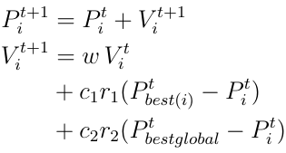
The particle's position P and velocity V in the design space are deduced from their values at the previous iteration according to the formula on the right.
The rate of change is the sum of three quantities based on:

1. the particle's inertia,
2. the knowledge of the personal best P_best that the particle remembers having achieved so far,
3. the information communicated by the rest of the swarm of the global best P_bestglobal that the swarm has achieved so far

The idea is that each particle tries to modify its current velocity to improve its personal best.

The respective importance of these three quantities is determined by three coefficients called the inertia weight w, the cognitive weight c₁ and the social weight c₂.

The inertia weight w is analog to the mass in mechanic: the greater the mass, the more force it takes to change the velocity.

r₁ and r₂ are random numbers in the range [0,1] intended to add diversity to the swarm movement.

Termination

The algorithm ends when one of the particle's fitness satisfies the objective, or when the maximum number of iterations has been reached.

Muti-Objective Particle Swarm Optimization

Principles

The MOPSO algorithm is an extension of the PSO and uses the same principle. The main difference is that there is no unique or simple definition of "the best" particle in the swarm since the distances to each of the objectives may be measured differently and cannot be compared.

To illustrate this, consider the optimization of a plane for the two simultaneous objectives |Cm| <ε and Cl/Cd ≥ 30 at a specified angle of attack. A pitching moment coefficient cannot be compared to a glide ratio, and the algorithm cannot determine by itself which of the two objectives is more important. Also there is usually no unique best configuration which satisfies all objectives, but instead several different solutions may satisfy both objectives.

The standard method to select the best particles is to build the Pareto front (or frontier) of the swarm, and to retain those particles which are non-dominated.

Similarly to the single objective PSO, the algorithm ends when one particle satisfies all objectives, or when the maximum number of iterations is reached.

PSO 2d demo and proof of concept

Demonstrator

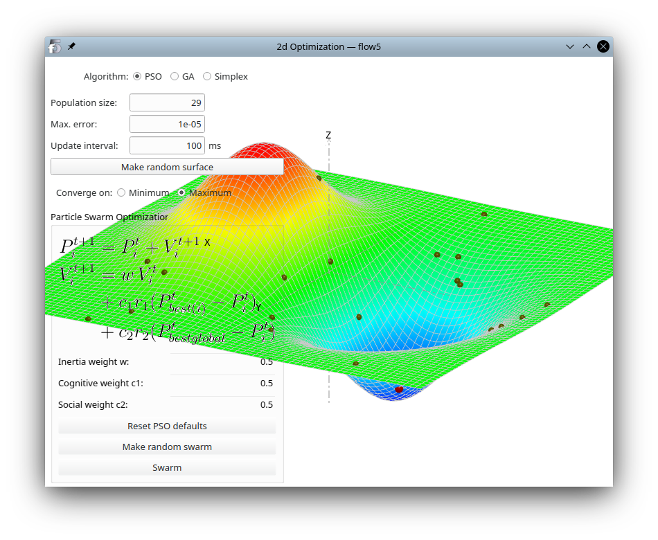
A 2d visual demonstrator of the PSO and GA algorithms can be accessed in flow5 using the keyboard shortcut Ctrl+N and F11.

This demonstrator can be used to test the influence of the algorithms' key parameters.

Proof of concept

As a proof of concept case, a PSO module has been implemented in flow5 to optimize a foil's shape to achieve a given inviscid pressure distribution.
As it turns out, the PSO converges robustly towards the target distribution.
The module can be accessed by switching to the Foil design module, selecting a foil, and using the keyboard shortcut F11.

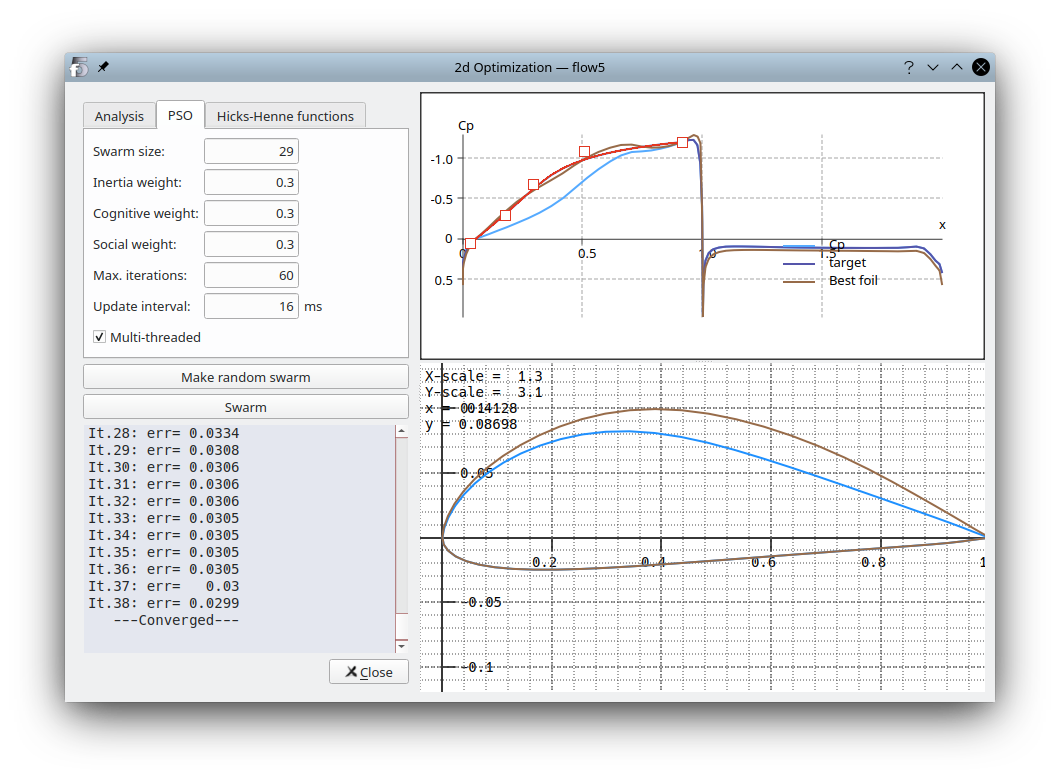
The module is provided for information only and is of no practical use. It offers no advantage compared to XFoil's MDES and QDES modules. The goal was to determine the potential applicability of the PSO to the analog 3d case.

Application to airplane optimizations

The MOPSO implemented in flow5 is the basic version of the algorithm, with the additional tweak of random particle regeneration each time the swarm moves.

Many improvements and variants of the algorithm have been published over time, and some of these variants may be evaluated in the future and included in flow5 if a benefit is seen.

As it is, the module is stable, operational and can be used to perform optimizations.
As of flow5 v7.07 however it is provided for user testing and feedback, since the interface lacks maturity and since the module may not address all user needs.
Depending on its potential utility a scripted optimization module may be added in a future version.

Objectives

The objectives which can be selected are:

1. the lift coefficient
2. the total drag coefficient
3. the glide ratio Cl/Cd
4. Cl^3/2/Cd
5. the pitching moment coefficient Cm

Other design objectives may be added to the list on request.

Design space

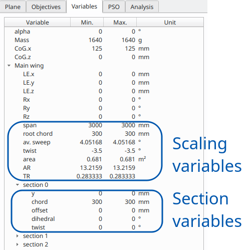
The module can be used to optimize an internal xfl-type plane. An illustration of the design variables is given in the image on the right.
Any number of design variables may be activated for a given optimization run.

Up to v7.13, a wing's geometry could be optimized using the scaling variables which are the span, the root chord, the average sweep, the twist, the area, and the aspect and taper ratios. Starting with v7.14, the section variables can be activated individually.
Note that activating simultaneously variables of each kind will create a conflict with unpredictable results. This could occur for instance when activating the span range variable and y-positions of one or more sections.
The recommended way is to optimize first using the scaling variables and to switch to section variables only for a more refined optimization.

Important notes

• The objectives are expressed as target values with a maximum acceptable error. The algorithm does not handle naturally requests to maximize or minimize a fitness function because the swarm has no way of knowing whether it has reached the position of maximum or minimum in the design space. The method to maximize an objective is to set it to a high target value. Optimization will end when the maximum number of iterations has been reached.
• The number of design variables activated for an optimization run should be at least equal to the number of objectives. The greater the number of variables, the greater the chances are of converging towards a solution.
• To increase the chances of convergence, the design variables to activate are those which have the largest impact on the objective.
• An optimization problem may not have a solution in the given design space. This can occur for instance when requesting an excessive glide ratio which cannot be achieved even with the design variables hitting the boundary. In fact since by nature the goal of optimization is to test the limits of the design space, this situation is likely to occur.
  
• Another potential cause for failure to converge is the incompatibility of objectives. For instance targeting both a lift coefficient and a glide ratio for a specified a.o.a. is likely to be inconsistent.
• The weight coefficients have a strong influence on the convergence rate of the MOPSO. It is recommended to experiment with the 2d demo to understand their influence.
• An additional probability of regeneration has been added to the core MOPSO algorithm, so that each particle has a random chance of being randomly repositioned each time the swarm moves. This introduces diversity in the swarm and tends to improve convergence in the case of low swarm sizes. This probability should be kept at a low level, typically 5%.
• To reduce the optimization times and increase the chances of success, it is best to perform limited incremental optimizations of the selected plane.
• Constraints are treated as objectives. For instance constraining the pitching moment coefficient to zero is equivalent to setting a design target Cm=0 with a tolerance.
• The angle of attack is treated as a design variable.

Restrictions

• Only models without a fuselage should be selected for optimization. The reason is that the fuselage and wing meshes cannot be automatically adjusted for each state of the design variables.
• It is important to keep in mind that the algorithm performs a great number of calculations of operating points, i.e. one for each particle at each iteration. To limit the duration of the optimization process, only small meshes consistent with low analysis times should be used.
• The flap positions are not (yet?) included in the design space. The main show-stopper is the impossibility to evaluate the viscous drag on the fly for each flap position.
  The flap positions may be added in a future version for inviscid optimizations.

Step-by-step

Start configuration

Incremental optimization

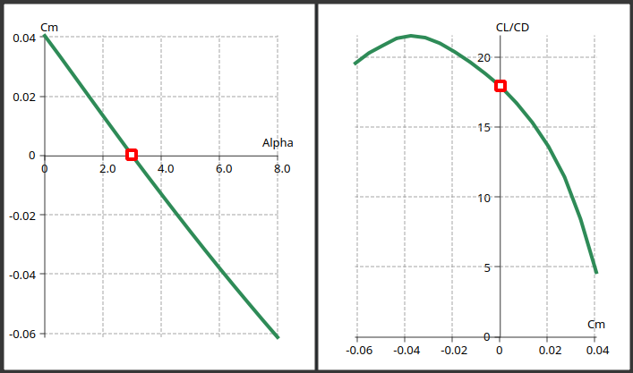
Experience so far has shown that the MOPSO algorithm works best by optimizing incrementally an existing plane. The subject plane should be analyzed and the reference performance points, e.g. lift coefficient or glide ratio, should be determined and used as the starting point.

In the case illustrated in the image below, the current glide ratio is 18 at the aoa 3° for which Cm=0. A reasonable optimization problem could be to achieve Cl/Cd = 21 in the range [2°-4°] with the constraint Cm=0.

Consistency of objectives with design variables

The design variables should be selected for their influence on the ojectives. In this case they are chosen to be:

• the angle of attack
• the main wing's aspect ratio
• the main wing's twist

Mesh size

Since the MOPSO performs a very large number of calculations, it is important that each calculation runs in a fraction of a second. This implies that the mesh size in particular should be small, and how small depends on the platform's computing power.
Typically the analysis configuration should be:

• a few hundred panels at most
• thin surfaces
• uniform triangles or quads
• no viscous loop
• no fuselage
• T1/2 analyses

Fine optimization of the model with more complex meshes and analysis types should be performed manually after the automatic optimization has determined the best qualitative solutions.

Interface

The optimization module is accessed by selecting the plane to optimize, then using the context menu action "Active plane/Optimize" or the keyboard shortcut F11.

The settings of the analysis and of the MOPSO algorithm are presented on the left side of the interface and the results on the right side.

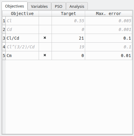
Objectives

The objectives are defined in the first tab of the left column.
The key points to check are that

• the target values can be realistically achieved in the design space.
• the objectives should not be set inconsistently; for instance targeting more than one of the objectives Cl, Cl/Cd, and Cl^3/2/Cd may be possible, but will most often fail if the design space is not large enough.
• the max. error should not be too small, otherwise the particle may miss the target by a fraction and then "swarm away".

If the intent is to maximize an objective such as the glide ratio, the target value should be set to a high unrealistic value. In such a case, convergence cannot be achieved and the optimization will end when the maximum number of iterations has been reached. The solution to keep can then be selected manually in the Pareto frontier.
Similarly, to minimize the drag, set its target value to zero.

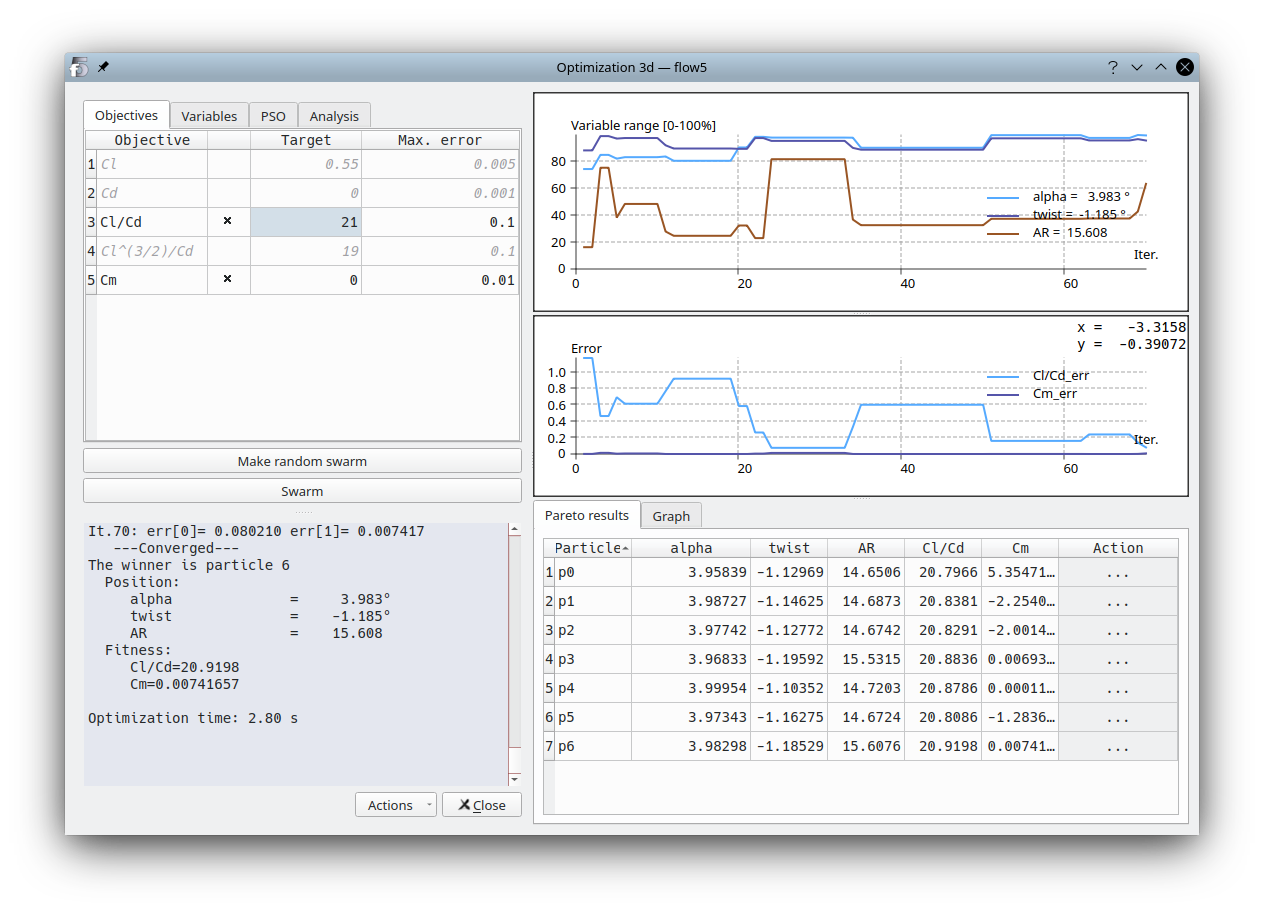
In the case illustrated in the image on the right, the objective is to achieve Cl/Cd = 21 with maximum error 0.1 together with the constraint Cm=0 with maximum error 0.01.

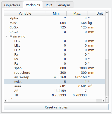
Variables

A variable is activated by selecting different minimum and maximum values.
There is no limit to the number of variables which can be activated. The important thing is that the variables to activate and their range should be chosen so that they are consistent with the objectives to reach.
Increasing the number of variables may improve the chances of finding an optimal solution, but may also cause the algorithm to wander a little more. Experimentation is still on-going to establish guidelines.

The variables are inherently plane-dependent, so that a set of variables is kept in memory for each plane for the time of the session. The variables are not saved to the project file.

In the case illustrated in the image on the right, the design variables which have been activated are:

• angle of attack in the range [2°, 4°]
• main wing's twist in the range [-5°, -1°]
• main wing's aspect ratio in the range [13.2, 17]

MOPSO parameters

The convergence and robustness of the MOPSO algorithm are very sensitive to the value of the parameters, which should only be modified with care. Also, experimentation is still on-going so that the recommendations and default values may change in the future.

Swarm size

The number of iterations to convergence decreases with the swarm size, but each iteration will take longer. Experimentation so far seems to show that a swarm of 30 particles is a good starting point.

Max. Pareto size

This parameter defines the maximum number of non-dominated solutions that can be stored in the Pareto frontier. It has been added since it is recommended in publications to control this size, but experimentation so far seems to show that it makes little difference on the convergence. By default this size is set to 10 particles.

Inertia, cognitive and social weights

These weights condition the particles' change of velocity each time the swarm moves. There are widely different published recommendations for these weights so that it is delicate to give guidelines. The best results so far have been achieved with w=0.3, c₁=c₂=0.7;

Regeneration probability

Although this parameter is not present in the original core PSO algorithm, it turns out that it can be useful to add diversity in case of low swarm sizes. Too high a value will cause the swarm to scatter and wander aimlessly, too low a value and the swarm will get stuck on a non-optimized value within a few iterations.
It is recommended to leave this parameter at its default value of 5%.
It can be increased with precaution in cases where the swarm tends to get stuck too easily on local optimums instead of converging on the global best position.

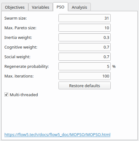
In the case illustrated in the image above,
the parameters have been set at their default values.

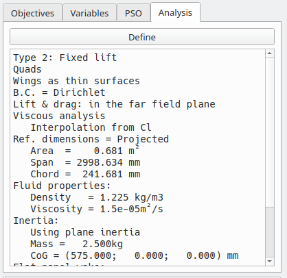
Analysis

By default, the analysis set for the MOPSO is the last one defined in the plane module. The analysis settings can be modified by clicking the "Define" push button.
It is strongly recommended to use a simple type of analysis to limit the computation times, e.g.

• Type 1 or 2
• Thin surfaces
• Uniform density quads or triangles

Note that the inertia will automatically be set to manual and the plane's point masses will be cleared so that the mass and CoG position can be used as design variables.

Optimization run

Once the input data has been defined, click on the "Make random swarm" button, and wait for a confirmation message in the output pane that the Pareto frontier was successfully built.

Press the "Swarm" button to start the iterations. The algorithm can be interrupted by pressing this same button again, and can be resumed by pressing it another time.

Note that if the algorithm ends or is interrupted without convergence, the Pareto frontier will still be displayed in the bottom right table, however none of the particles will meet all objectives.

If the MOPSO failed to converge, it is possible to either:

• restart the iterations from the swarm's last position by pressing again the "Swarm" button,
• generate a new ramdom swarm and press the "Swarm" button.

Lastly, the swarm should be regenerated manually each time the selection of objectives has changed. If only their values have changed, regeneration is not necessary.

Results

The results are presented on the right side of the interface.

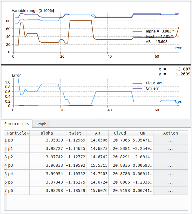
Best particle position

Since there is no single best particle but instead several which constitute the Pareto frontier, flow5 selects for display the best particle with minimum normalized distance to the origin. The normalization is made by dviding the particle's error by the objective's maximum admissible error. This particle is highlighted in red in the Pareto graph.
The top right graph plots its position in a normalized space at each iteration. It may illustrate which variables have influence and which variables tend to remain constant or inversely tend to hit their boundary.

Best particle fitness and error

The middle graph plots the error of the same best particle with regard to each objective. It may illustrate which objectives remain out of reach in the design space.

Pareto frontier

The bottom table lists the particles in the Pareto frontier at each swarm iteration. Only one of these particles may meet all objectives, and only if the algorithm has converged. The index of the winning particle is given in the text output in the bottom left pane. In the present case the winner is particle p6 which meets all the objectives.
The particles may be sorted by clicking on the column headers.
Click on the three dots in the Action column on particle p6's row to save the plane to the project file.

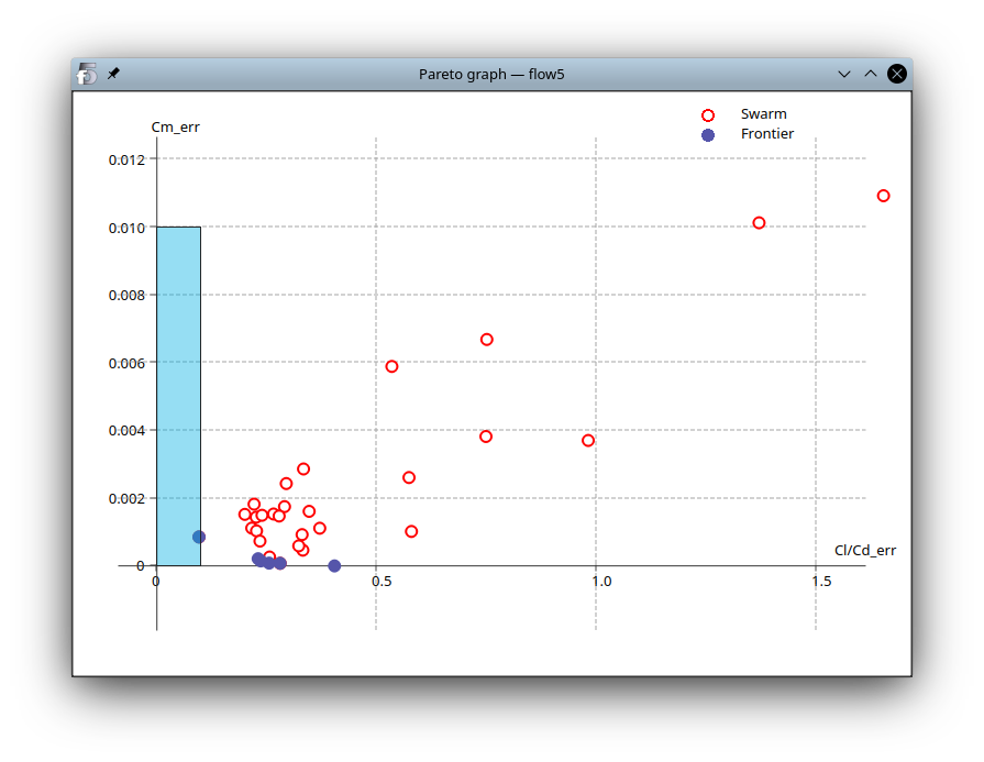
Pareto graph

In the case of an optimization run with two and only two objectives, it is possible to view the Pareto graph in the bottom right tab. The graph is updated after each iteration, which may help to visualize the swarm's convergence towards the target rectangle.
Each circle represents a particle, with the filled purple circles constituting the frontier.
The target rectangle is overlayed in blue.

The optimization target is reached when one particle enters the rectangle.

Note that the number of particles in the frontier is limited to the maximum size defined in the "PSO" tab, so that some particles which should be in the frontier are sometimes excluded.

Resuming the optimization

It is is possible to change the values of the design variables and the target values of the objectives and to start a new optimization without regenerating the swarm. Note however that the swarm may lack diversity and that convergence may not be better than by starting with a fresh swarm.

If the selection of objectives has changed, e.g. targeting a lift coefficient instead of a glide ratio, the swarm must be regenerated.