3d Inverse design
Updated April 17, 2021
------------------ WORK IN PROGRESS ------------------
Background
flow5 v7.09 introduces a new module to perform the 3d inverse design of foils, with the goal to achieve specified Cp profiles at the main wing's sections. Although the goal is similar to those of XFoil's 2d MDES and QDES modules, the method used is fundamentally different and is based on the MOPSO algorithm.
As of flow5 v7.09, the feature is stable and usable. It is however still experimental and has been activated for testing and feedback.
Problem specification
The module is designed to achieve specified pressure distributions at the wing's sections. Additional objectives targeting lift and other aerodynamic coefficients may be added to future versions.
Methodology
The inverse design process uses the following building bricks.
Specification of the target Cp profiles
The profiles are specified using B-Splines in a manner similar to the method already implemented in xflr5's inverse design module. This method has the advantage of simplicity and versatility.
The Cp profiles are specified at each of the wing's section, with the exception of the tip section where the evaluation of the Cp coefficients is too imprecise for use.
There is no limit to the number of sections at which the Cp profiles can be specified. Increasing the number of sections will provide more control on the target values, but may also run the risk of over-constraining the optimization. For this reason it is important to ensure that the profiles specified at all the sections are reasonably consistent.
The time to move the swarm at each iteration will not increase significantly with the number of sections, but it may cause it to wander a little more before convergence.
If a spline is not defined at a given section, the Cp profile is assumed to be free.
Foil parameterization
Several methods have been developed and proposed over time to describe the shape of an airfoil. Cf. for instance "Parameterization of Airfoils and Its Application in Aerodynamic Optimization", J. Hajek, WDS'07 Proceedings of Contributed Papers, Part I, 233–240, 2007.
The method implemented in flow5 is the Hicks-Henne description based on bump functions. This method has given good results in 2d and has been selected for the 3d extension. Other parameterizations will be tested and added if a benefit is seen.
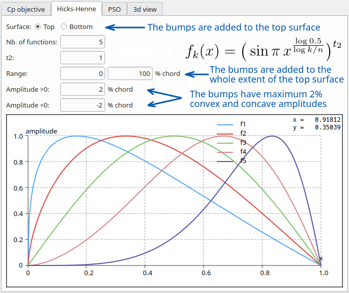
The bumps are described by the following set of functions with k ranging from 1 to n:
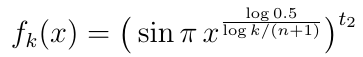
The maximum bump of function fk is located at the fraction k/(n+1) of the chord. The width of the bump is controlled by the parameter t2.
The shape of the functions is illustrated in the image of the right for n=5 and t2=2.

MOPSO algorithm to achieve the target distribution.
The algorithm is common to the one used for the optimization of plane configurations and is described here.Transpiration technique
This method allows the fast generation of an approximate solution to a panel problem. Its intent is to avoid the very lengthy generation and factorization of the influence matrix at each time step and for each particle.
A detailed description of the transpiration technique falls outside the scope of this document.
Its main idea is to add to the boundary conditions a normal blowing velocity which is adjusted to make the flow tangent to the desired modified geometry.
The method remains relatively precise as long as the modified shape does not deviate too much from the base shape, and as long as the streamwise step between two nodes remains small especially in areas of large pressure gradients.
Note: The use of the transpiration technique requires the additional storage in memory of a source influence matrix 1/6 the size of the doublet influence matrix.
Limitations and restrictions
Linear thick surface method
The inverse design is only implemented for the linear Galerkin method applied to thick surfaces. The reason for this limitation is double:
- it enables and simplifies the specification of Cp profiles along streamwise strips of nodes,
- the linear order provides better accuracy at the leading stagnation point where the pressure gradient is high.

Fuselage
To enable the use of the transpiration technique, and because it is not possible to re-mesh the fuselage-wing junction for each particle, only configurations without a fuselage, or where the fuselage does not connect to the main wing should be used.
Main wing
To keep the UI and process simple and because the optimization of secondary wings such as the elevator and the fin are of lesser interest, the parameterization of sections is only activated for the main wing.
The wing should be symetric, i.e. with the same foils on the left and right sides.
Inviscid analysis
Since the viscous data cannot be generated on-the-fly for each particle configuration, only inviscid optimization is activated.
Future developments
Depending on the interest for the module and the feedback, additional design variables and objectives may be included in the optimization process.
Design variables
- Alternative parameterization methods for the foils
- Wing section data such as twist and dihedral
- Foil flap positions
Design objectives
- Lift, drag and other aerodynamic coefficients
Back to top
Step-by-step
The project file used in this example can be downloaded here: 3d_inverse.fl5.Start configuration
Since the goal is to achieve optimization by modification of a base configuration, i.e. by incremental changes, starting from a base configuration close to the target configuration will improve the chances of convergence. It will also reduce the error implicit in the use of the transpiration technique.
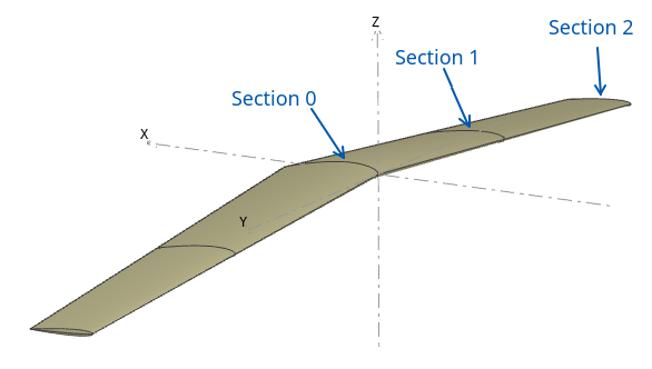
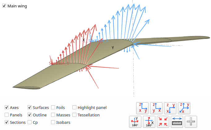
The test case is a pseudo AC75 type foil with inverse dihedral, defined by three sections. The sections are numbered starting with section 0 located at the root section. Section 2 located at the tip is excluded from the optimization process.
It is a good precaution to run a tri-linear thick surface analysis at the desired a.o.a. prior to launching the optimization module, and to check that the Cp profile at sections is smooth and is a good basis for optimization.
Optimization setup
Interface
The module is launched by selecting the test plane, then activating the context menu option "Active plane/Inverse design", or by using the keyboard shortcut Ctrl+F11. This will open the interface of the optimization module.
The input data for the optimization task is defined in the left column and the results are presented in the right column.
Target profiles
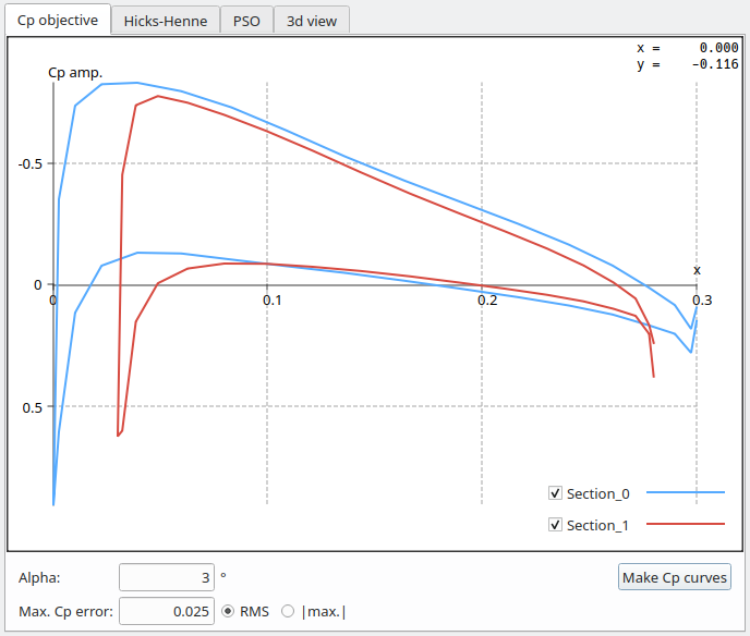
In the "Cp objective" tab, enter the desired a.o.a. and click "Make Cp curves". The analysis will be automatically set to the tri-linear, thick surface, inviscid type.
The Cp curves at the sections will be displayed both in the graph view and in the 3d view once the analysis is completed.
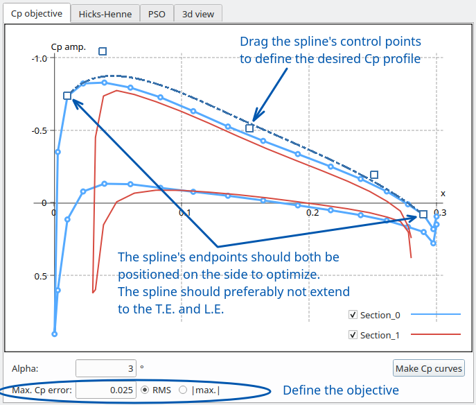
Activate the checkbox of a section to optimize, then click on the curve. A spline with endpoints located by default on the x-axis will be shown.
Drag the spline's control points to define the shape of the desired Cp profile.
As with all graphs in flow5, hold the 'X' or 'Y' key down while scaling to expand that axis only.
Important notes:
- The spline's endpoint must be located on the reference profile curve.
- The spline's endpoint should be located at points located on the same side of the foil.
- Specifying the profile in the areas of the LE and TE should be avoided because of the high pressure gradient and its induced high influence on the transpiration method.
- To cancel the objective at a section, use the context menu option (i.e. Right click) "Reset spline/spline #"
The last thing to do before exiting the tab is to define the maximum acceptable error for the deviation of the Cp profiles at each section.
The cumulated deviation is measured from one spline endpoint to the other.
It is possible to start with a large value and reduce it progressively without need to re-create the swarm
In the present case the maximum deviation is set to RMS = 0.025. Experience so far seems to show that the deviation should be specified as an RMS value rather than a |max.| value.
Hicks-Henne bump functions
In the "Hicks-Henne" tab, select the side to which the bumps should be added. For maximum effect, the bumps should typically be added to the same surface as the one for which the target Cp was set. In this case this is the top side.
The amplitude should be set to a value sufficient to achieve the desired target profile. Too large a value however will cause imprecision in the transpiration technique and may cause the swarm to wander.
Experience so far has shown that the number of functions should preferably be kept low, e.g. less than 5, with large overlaps, i.e. t2<2, to avoid bumpy foil shapes and to obtain smooth Cp profiles.
In the present case:
- 5 bump functions are applied to the whole extent [0%, 100%] of the foil's top surface,
- a maximum symetric amplitude equal to 2% chord length has been set. Setting the minimum amplitude to 0% will eliminate the risk of concave foil shapes, but runs the risk of reducing excessively the design space.
Important note: The range of the bumps should be similar to the range of the splines.
- If the range of the bumps is too small, the target Cp profile will not be achievable in the part of the surface which is not covered by the bumps.
- If the range of the bumps is greater than the range of the spline, the amplitude of the outer bumps will be unconstrained and will lead to wavy foil surfaces.
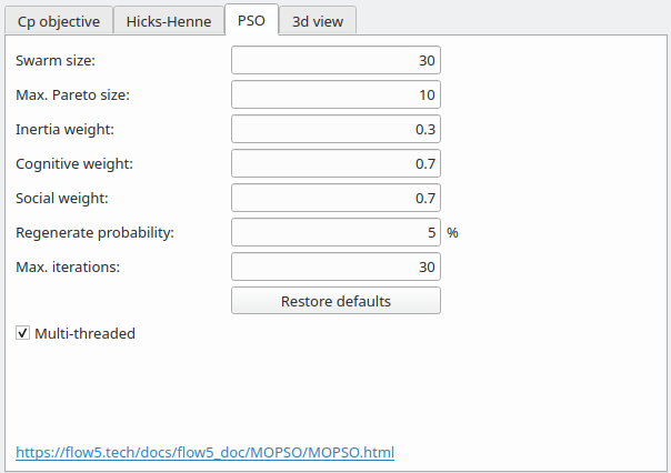
MOPSO parameters
These parameters should preferably be left unchanged, except for the swarm size and the max. number of iterations which can be adapted to the speed of the platform and to the size of the mesh.
The detailed explanations and recommendations are given here.
Optimization
Click on the "Make random swarm" button and wait for the build task to finish. The task cannot be interrupted.
Click on the "Swarm" button. If the swarm does not yet exist, or has become invalid due to a change of parameters, a message will be shown requesting to build or rebuild the swarm. Otherwise the optimization process will launch.
The iterations can be interrupted at any time by pressing again the button.
Optimization results
Output views
The convergence of the swarm can be controlled in the bottom right text pane and in five graphic outputs:
- 2d and 3d Pareto graph
- Swarm iterations graph
- Cp graph
- Foil view
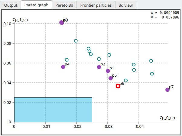
Pareto graph
At each iteration, the algorithm selects the particle in the Pareto frontier with the minimal distance to the origin, and displays this particle in all the views.
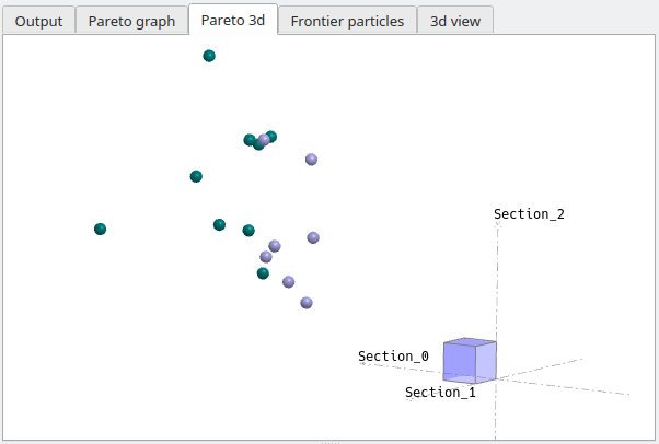
The Pareto graph has a dimension N equal to the number of sections where splines have been defined. However it can only be displayed in 2d for the first one or two sections, and in 3d for the first three sections.
In the present case, particle p6 highlighted in red is the best particle, i.e. the one closest to the origin.
Convergence is achieved when a particle enters the blue rectangle. Note that the particle's position at the sections not represented in the Pareto graph also need to enter the blue rectangle, cube or "N-hyper cube" for convergence to be achieved.
In the case illustrated in the right graph, the target error has been reached at section 0, since particle p4 for instance has Cp_0_error < 0.025, but not at section 1.
See the paragraph non convergences for common causes and fixes.
Swarm iterations
The RMS-deviations of the Cp profiles to the target profiles are displayed in the middle right graph as a function of swarm iterations.
The iterations can be interrupted and resumed at any time. It is possible to re-start iterations from the current swarm, or by first re-generating a new random one if the swarm seems to be stuck on a local minimum.
Results are generated whether the optimization process has converged or not.
In the present test case, convergence was achieved at the first run in 12 iterations.

Non convergence
It often happens that the algorithm does not converge, i.e. stagnates at a certain distance from the objective at one or more section. The cause of non-convergence can most often be identified in one of the outputs, so it can be a good idea to interrupt the task and to check the graphs and views for potential issues.
Typical causes of non convergences are:
- A solution cannot be found in the design space. This may occur for instance if the chordwise range of the bump functions does not cover the whole range of the splines. In fact it is recommended to always set the range of the bump functions to [0, 100%] unless there is a good reason not to.
-
The swarm is stuck on a local optimum, or lacks diversity. This can be seen in the Pareto graph, where the frontier particles are grouped and remain stationary at each iteration.
The fix is to make a new swarm and restart the iterations. -
The difference between the target Cp and the calculated Cp can be quite large in the area of the leading edge due to the local high pressure gradient, thus maintaining the error at a high level.
For this reason, it is recommended to avoid setting the spline's left point at the L.E. or close to the L.E..
The same goes for the T.E.. - The t2 parameter of the bump functions is too large, causing the bump functions to not overlap sufficiently.
- The specified profiles at adjacent sections are not compatible, e.g. requesting a pressure increase at one section and a decrease at the next is likely to fail.
- The chordwise number of panels is insuffient and does not provide enough degrees of freedom. The fix in this case is to exit the module, and to increase the wing's surface mesh density.
- The value of the objective is too low.
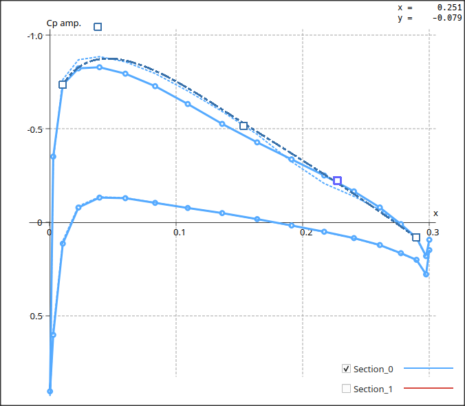
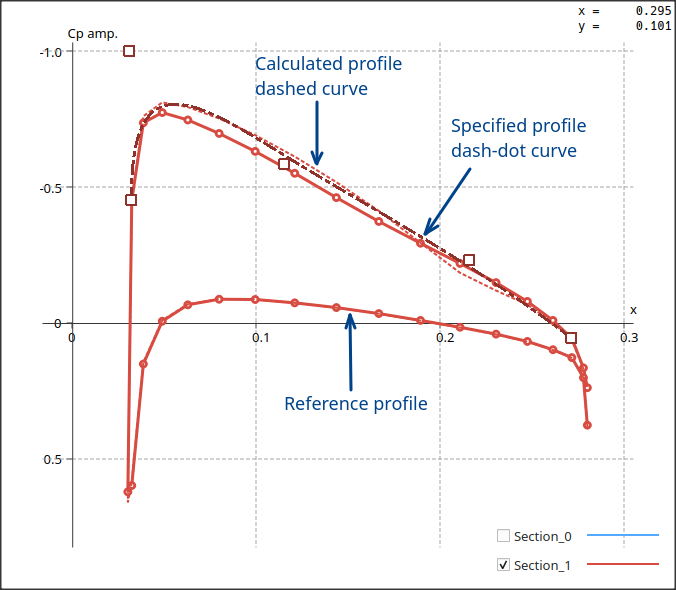
Cp profiles
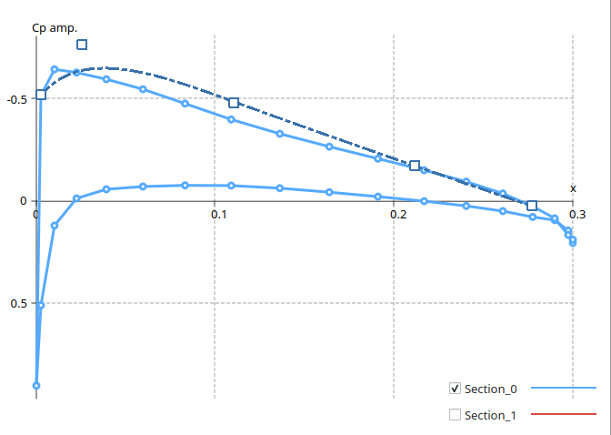
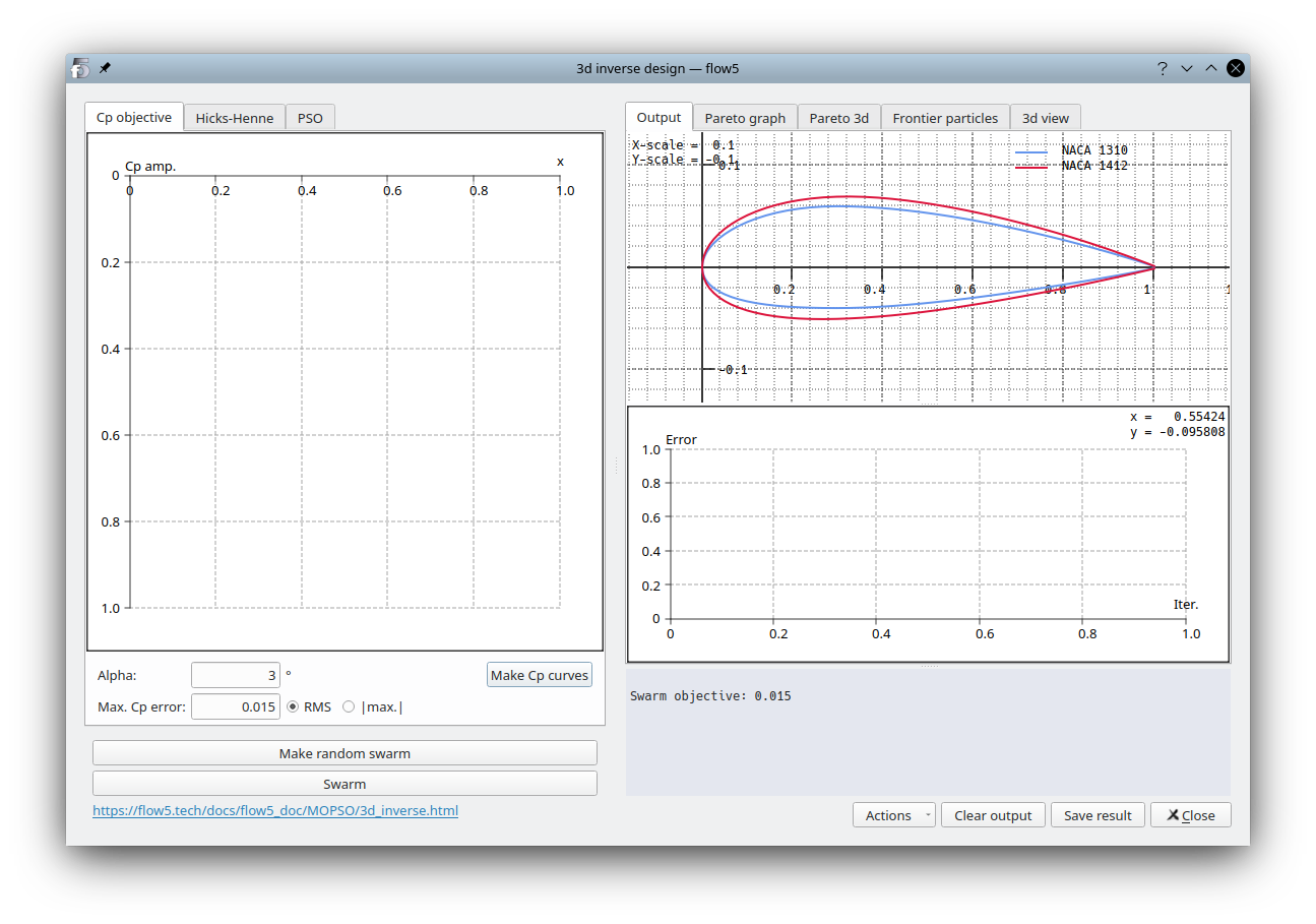
The optimized profiles are overlayed on the top left graph as dashed curves.
Foil shapes
The optimized foil shapes are displayed in the top right view.

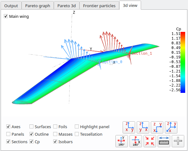
3d isobars
For information, the resulting Cp colour maps and the isobars are displayed in the top right 3d view.
Store the result
If satisfied with the result, click the "Save result" button and exit the module.
Optional sanity check
Since the optimization process was conducted using an approximation implied by the transpiration technique, it can be interesting to compare the results to the exact solution of the panel method.
This is done after exiting the module by defining a tri-linear analysis for the optimized plane, runnning the analysis for the specified a.o.a., plotting the results in the Cp view (F9), and overlaying manually the optimized curves using the "External curves" feature.
As it turns out, the error due to the approximation is negligible.
The slight offset of the red curves at section 1 is caused by the profiles not being evaluated at exactly the same span position, and it is not significant.
