The Vortex Particle Wake

Updated September 22, 2020

------------------ WORK IN PROGRESS ------------------

Back to main table of contents

Theory

An interesting alternative to the modeling of the wake by flat panels is the Lagrangian description based on discrete vortex particles.

A theoretical description of the Vortex Particle Wake (VPW) can be found in the following documents:

An unsteady, accelerated, high order panel method with vortex particle wakes, D. J. Willis, M.I.T. 2006.
A combined pFFT-Multipole tree code, unsteady panel method with vortex particle wakes, D. J. Willis, J. Peraire, J.K. WHite, 43rd AIAA Aerospace Sciences Meeting and Exhibit, 10-13 January 2005, Reno. N.V.
A boundary element-vortex particle hybrid method with inviscid shedding scheme, Y. Wang, M. Abdel-Maksoud, B. Song, Computers and Fluids 168 (2018) 73–86.

David J. Willis's work is complete, well presented, and is, to my knowledge, the first comprehensive example of a VPW implementation. The second document provides a good summary of his methodology. You can ignore the math and have a look at the figures to get an idea of how it works.
The third document provides useful practical details on the numerical implementation.

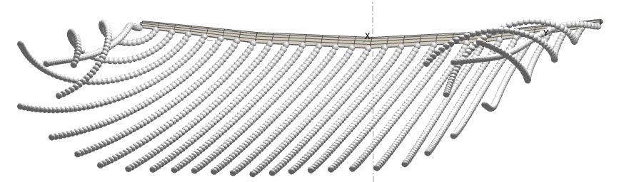
The idea of the method is to:

Move from a Eulerian to a Lagrangian description of the wake
Represent the wake by discrete lumped vortices, or "vortons", instead of flat panels with distributed doublet densities.
Build the wake incrementally by advecting the vortons as the wake unfolds downstream.
Add the contribution of these vortons as an added term to the RHS vector of the potential flow's linear system.

This approach offers several advantages which make it attractive for an implementation in a panel solver:

It solves the problem of self intersection of wake panels.
It can be used as a body piercing wake, which solves the problem of wake panels intersections with the body.
It offers a natural implementation of the vortex core radius, to account for the viscous behaviour.

Implementation in flow5

The VPW model implemented in flow5 beta 12 is essentially the one described in the documents referenced above with the main following deviations.

The vortex viscous stretching and particle redistribution are not implemented (yet)
The vortons are translated downstream at each step by a fixed length instead of using a time-dependent scheme
The quadratic panel method is not implemented.
Since even uniform methods can provide potential solutions within 1% accuracy, higher orders do not seem justified. What's more, the error on lift and drag due to the inviscid assumption and to the simplified wake model is expected to be one order of magnitude higher. This makes the need for methods of higher order even less likely.
The acceleration algorithms are not implemented (yet)

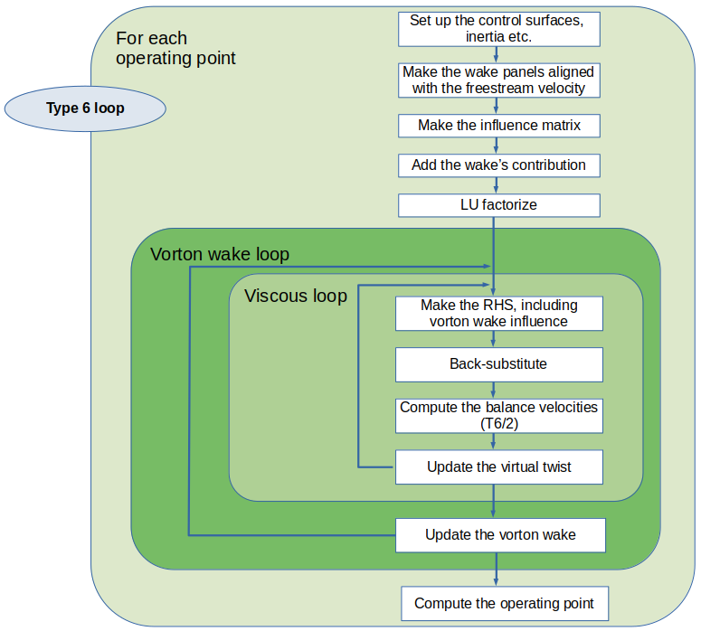
Potential solution

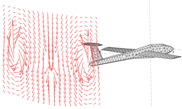
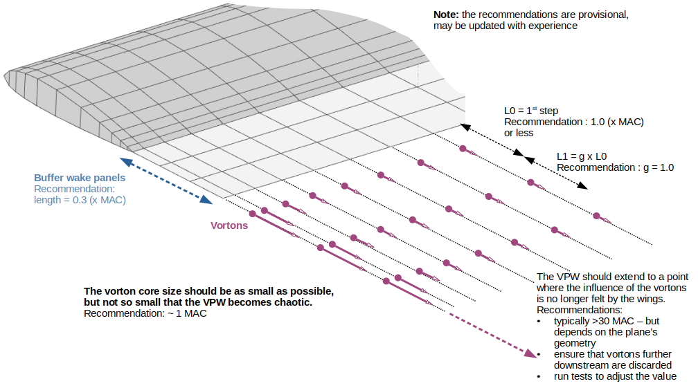
The potential part of the wake is made of 3 rows of "buffer wake panels" ended by a "negating vortex" which cancels the end effect of the last downstream wake panel.

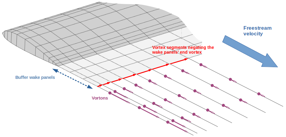
The buffer wake panels are aligned with the freestream flow for each a.o.a. calculation.
The procedure used to convert the buffer wake panel's vorticity into vortons is essentially the one described in the third reference document.

Vorticity

Each vorton is described by its position in space and its vorticity vector. The amplitude of the vector is the vorton's circulation which is set when the vorton leaves the trailing wake panel.

Each vorton induces a velocity field. To avoid the velocity from going to infinity close to the vorton, a "mollification" or damping factor is applied to the velocity vector. This mollification factor is described in the third reference document. It is illustrated in the figure below for a core size = 100mm.

The recommendation of the authors is to set a core size no less than inter-particle spacing, which implies that this core size may need to be adjusted depending on the model's mesh and the buffer wake's settings.

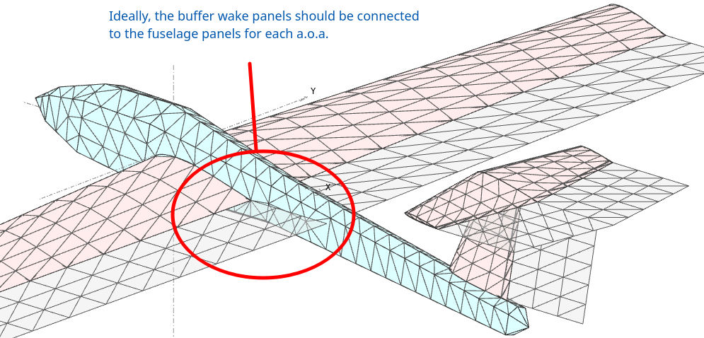
Mesh

It is recommended in the first reference document to adapt the body's mesh and the buffer wake panels so that the elements share a common edge. This is intended to avoid numerical problems and to have a "body abutting wake".

However this also means that the fuselage would need to be re-meshed for each angle of attack, which is not practical. For this reason, the wake panels are aligned with the freestream flow for each angle of attack, and the numerical interactions between these panels and the fuselage are tolerated until a better solution is found.

Analyses

With the introduction of the VPW, the problem becomes non-linear, and it requires the solution to the potential flow at each step of the wake development. For this reason, it is not compatible with the Type 1, 2, 3 and 7 analyses, and is only activated for the Type 6 control polars. The viscous loop iterations are nested in the development of the VPW. Note however that there are other options to organize the loops which can for instance be dissociated. Numerical experiments will help determine the best way to solve the problem and the loop's organization may be modified in future versions.

Convergence

In flow5 beta 12 the VPW loop ends when the maximum number of iterations is reached. Preliminary testing shows that the convergence is obtained after only a few iterations.

Loop exit conditions based on the convergence of the lift and induced drag coefficients may be added in future a version.

Induced drag

The evaluation of the induced drag is something very tricky in panel methods, and the result depends on the calculation method, on the wake representation and on its converged shape.

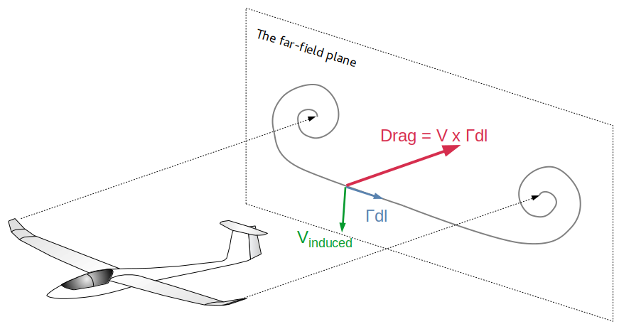
As stated by Mark Drela in "Flight Vehicle Aerodynamics", M.I.T. 2014, paragraph 5.6: "The induced drag expression is seen to be the crossflow kinetic energy (per unit distance) deposited by the body. This energy is provided by part of the body's propelling force working against the induced drag. The remaining part works again the profile drag."
The problem of estimating the induced drag therefore translates into the estimation of the kinetic energy in the crossflow plane. Given the chaotic nature of the streamlines for anything other than a simple standalone wing, this evaluation can be quite problematic.

The most direct way to evaluate the induced drag is by summation of the pressure forces acting on the plane. As numerical experience has shown, this is not without problems however. To quote Mark Drela in "Flight Vehicle Aerodynamics" §5.1.2: "If the streamwise D (drag) component were computed in this manner, it would be simply incorrect or very inaccurate. The main reason is that the D_pressure integral has relatively large positive and negative integrand contributions over the surface which mostly cancel []."

The usual recommended way to evaluate the induced drag is to apply the Kutta-Joukowski theorem to the trace of the trailing edge's wake in the far-field plane. Quoting again Mark Drela in "Flight Vehicle Aerodynamics" §5.6.3: "The overall far-field drag is relatively accurate, since it does not suffer from pressure drag cancellation errors which make near-field pressure drag calculation unreliable".
This is the default method used in xflr5 and flow5.

Lastly, some authors have tried the direct numerical integration of the kinetic energy in the cross flow plane. However like all infinite sums of slowly decaying kernels, this can lead to numerical errors and unreliable results depending on the way that the integral is calculated.

In the case of a complex plane geometry shedding a chaotic wake, it is not straightforward to tell which is the most robust and precise of the three methods. More numerical experimentation is required to reach a conclusion and a recommendation. Until then, the induced drag is evaluated in flow5 in the far-field plane using the second method.

VPW settings

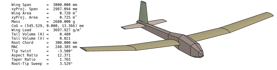
Sensitivity analyses have been performed on a simple case to establish tentative guidelines for the VPW settings. The project file used to perform these analyses can be downloaded here.

Influence of the wake's length

The wake's length influences the evaluation of the induced drag which is calculated in the far-field plane. This far-field plane is positioned by flow5 half-way down the VPW, so that both end effects are minimized.
The wake should therefore be sufficiently long so that the influence of the plane's elements is negligible half way down the VPW.
In the present case, the graph on the right shows that the evaluation of the induced drag does not change significantly for wakes longer than 30 MACs. Extending the wake further may improve slightly the accuracy of the analysis but comes at the expense of greater computation times.

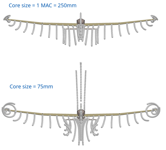
Influence of the core size

A critical parameter of an analysis involving a VPW is the vorton core size associated to the mollification function. The purpose of the mollification factor is to damp out numerical divergences which are caused by the absence of viscosity modelling in the analysis. The vorton core size can therefore be seen as an artificial or arbitrary correction factor, and as a consequence should be as small as possible to minimize this correction. However too small a size will cause the wake to become chaotic, and a too large size will excessively damp the wake's roll-up.

Since the vorton core size has a significant influence on the results, it has been moved from a global setting to an analysis specific parameter starting in flow5 v7.01 beta15.

The key reference dimension used to establish the vorton core size is the plane's MAC, in this case 250 mm.
This is the first value which should be tested for a given plane. If the analysis is stable, this value can be reduced progressively so long as the wake remains stable.
A good indicator of the stability of the roll-up is the smoothness of the polar curves. In what follows the induced drag coefficient is used as the indicator.

A first sensitivity analysis was performed with the following parameters:

Vorton core size = variable
Vorton streamwise step = 1 MAC

The induced drag coefficient is plotted in the graph on the right for various core sizes.
The analysis is stable, i.e. the curves are smooth, for core sizes down to 150 mm.

The difference of behaviour can also be seen in the shape of the vorton wake. The shape at the top of the image is for a core size equal to the MAC and at the bottom it is for a core size equal to 75mm. The diverging vortons in the latter case in the fuselage's wake show that the core size is too small.

Influence of the streamwise step

Another series of sensitivity analyses was carried out to evaluate the influence of the VPW streamwise step. As it turns out, reducing this step stabilizes the roll-up process.
The graph on the right shows the improvement due to the reduction of the step from 1 MAC to half a MAC for a core size equal to 50mm.
The reduction of the streamwise step comes at the expense of greater computation times.

Relation to the mesh's element size

Finally a last set of analyses has been run to determine if the core size should be adjusted to the width of the surface elements.
The number of spanwise wing elements was increased from 14 to 26 on each side, thus reducing the spanwise width of the wing's smallest surface element from 32 mm to 16 mm.
It can be seen that settings which ensure a stable wake for the coarse mesh (blue curve) are not good enough for the finer mesh (green curve).

In other words, the core size should be increased for decreasing element sizes.

Recommendations (still provisional)

VPW settings depend on the plane's geometry and on its mesh; the following recommendations are therefore guidelines which should be adjusted for each configuration.
Whatever the settings, make sure that the number of iterations is sufficient for the wake to extend at least thirty MAC downstream; run several analyses with different wake lengths to determine the optimal value such that the induced drag becomes independent of the wake length; discard the vortons further downstream to speed up the computation.
The main parameter to modify if the generated polar is not smooth, or if the VPW's shape is unstable is the vorton core size. To determine the appropriate value, run a first analysis
- with a core size equal to the plane's MAC,
- with the smallest streamwise step compatible with acceptable analysis times; this streamwise step should typically be smaller than the MAC.
Reduce the core size until the wake becomes chaotic or the polar curves lose their smoothness.
Consider smaller core sizes for finer meshes.