Building blocks of the panel method
Updated July 22, 2020
------------------ WORK IN PROGRESS ------------------
References
[1] Mark Drela, "Flight Vehicle Aerodynamics", M.I.T. 2014.
[2] David J. Willis, "An Unsteady, Accelerated, High Order Panel Method with Vortex Particle Wakes" M.I.T. June 2006.
[3] David J. Willis, J. Peraire; J. K. White "A Combined pFFT-Multipole Tree Code, Unsteady Panel Method with Vortex Particle Wakes.", 43rd AIAA Aerospace Sciences Meeting and Exhibit, 10-13 January 2005, Reno. N.V.
[4] Brian Maskew, NASA Report 4023, "Program VSAERO Theory Document, A computer program for calculating nonlinear aerodynamic characteristics of arbitrary configurations", 1987.
[5] James C. Sivells and Robert H. Neely, NACA TN-1269, "Method for calculating wing characteristics by lifting-line theory using nonlinear section lift data", 1947.
[6] E. Ting D. Chaparro and N. Nguyen, "Computationally Efficient Transonic and Viscous Potential Flow Aero-Structural Method for Rapid Multidisciplinary Design Optimization of Aeroelastic Wing Shaping Control", Advanced Modeling and Simulation (AMS) Seminar Series, NASA Ames Research Center, June 28, 2017.
Back to top
Building blocks
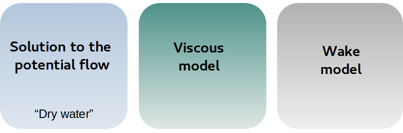 Panel methods such as those available in xflr5 and flow5 require three essential and independent building blocks
- A solution method to the potential flow problem
- A model for the wake
- A model for the viscosity
The goal of this chapter is to summarize what are the available options for each block, what are the choices made in flow5, and what they imply.
Back to top
A solution method to the potential flow problem
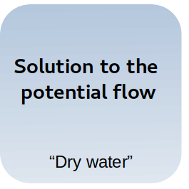
Of the three building blocks, the solution to the potential flow is the most straightforward. Laplace's equation is well understood and can be solved with a high degree of precision by using Boundary Element Methods (BEM), of which the panels codes used in aerodynamic calculations are a sub-case.
A comprehensive review of the development of panel methods is given by D. Willis in the introduction to his PhD work [2].
With time and experience, the preferred formulation has turned out to be the one based on surface source and doublet densities. It is the one described extensively by Brian Maskew in [4], and is the one implemented in xflr5 and flow5.
To some extent, there is a debate on whether linear and higher order elements are required for acceptable accuracy.
By nature, higher order methods using linear or quadratic densities on the panel elements are more precise than uniform methods. And while that is true, those higher order methods come at a computational cost that may not justify the benefit in increased accuracy.
Because the answer to this question is not straightforward, and that opposite points of view have been expressed on the matter, both a uniform and a linear order method have been implemented in flow5. For a time, the implementation of D. Willis' quadradic order method has also been considered.
As it turns out, the low order panel method is already remarkably precise with a reasonable number of surface elements.


D. Willis has pointed out in [2] that panel methods make most sense when the discretization of the surface is consistent with the order of the method. A linear method for instance uses three degrees of freedom compared to only one in the case of uniform methods, so that a linear method applied to large triangles is equivalent in complexity to a uniform method applied to three time the number of small triangles. However the latter option should be preferred for its more precise representation of the body's surface.
For these reasons the numerical experimentation with flow5 has led to the conclusion stated by Brian Maskew [4]: "This resulted in a push towards high-order formulation which, for subsonic flows at least, proved quite unnecessary".
As a conclusion to this paragraph, the uniform methods are more than good enough for a panel code designed to analyze bodies and lifting surfaces. The precision is less than 1% in the test cases, with a very reasonable number of surface elements. What's more, the error made in the two other building blocks is one order of magnitude higher than the error in the potential solution.
From a benefit to cost point of view, the uniform density methods are therefore recommended for use in flow5.
Back to top
A model for the viscosity
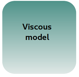
Of the three building blocks, the viscosity is the most difficult to implement.
Without viscosity, the panel method is a solution to "dry water" flow.
With the viscous assumption included, the problem becomes hugely complex and can only be adressed with RANS type flow solvers, or by using Interactive Boundary Layer (IBL) methods.
Such a coupling with an IBL is proposed by B. Maskew in [4]. This however adds a layer of complexity to the flow solver, and has not been deemed pracctical for applications such as xflr5 and flow5.
flow5 uses this same approach for the simple linear analysis types.

It accounts for moderate viscous effects and it comes at a reasonable computing cost with good convergence properties. It is therefore the model retained in the non-linear analysis types in flow5.

Back to top
A model for the wake
The wake is an integral part of the flow of lifting surfaces. The lift for instance can be seen as the reaction to the variation of vertical momentum transferred to the fluid, and the work of the induced drag is the kinetic energy in a crossflow plane. From the numerical point of view a wake model is required for lifting surfaces to implement the Kutta condition, and to obtain correct lift and drag loads on the surfaces. A panel method without a representation of the wake would be incomplete and incorrect.
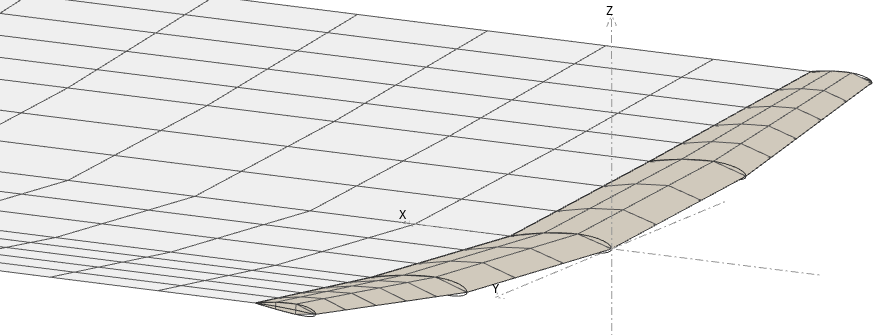
The flat wake model
In the simplest form of the Lifting Line Theory (LLT) and the Vortex Lattice Method (VLM), the wake is represented implicitely or explicitely by straight vortex lines extending downstream along the x-axis.
Similarly, panel methods in their simplest form make use of a flat panel wake. Here too the panels extend downstream from the lifting surfaces' trailing edges and are aligned with the x-axis.
In the case of uniform density panels, it can be shown that this representation is mathematically equivalent to the straight vortex lines used in the VLM.
This representation of the wake is commonly used in VLM codes and in panel methods, and it has proved to provide acceptable accuracy for most usages. From the numerical point of view, is has two advantages:
- It makes the problem independent of the a.o.a., so that the linear system can be built once and solved for the unit solutions; operating points for all a.o.a. can be calculated by linear combinations to save time and computations.
- The wake shape is prescribed once and for all at the outset of the calculation, and the solution does not require any iteration loop.
On the other hand, the model is not without its problems:
- Since the vortices or the wake panels are aligned with the x-axis, the analyses are limited to conditions of small angle of attack and low side slip angles.
- The vortex lines or flat panels are not "relaxed", i.e. they do not take the shape of the streamlines as they should. This implies that the wake is not a force-free surface as it should be, it carries loads, and it induces numerical parasite loads on the lifting surfaces
- The panels which extend from the trailing edges of the upstream surfaces may intersect or interact numerically with the downstream panels, which leads to numerical issues.
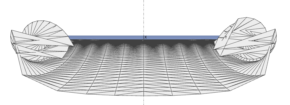
Wake relaxation
At the next level of complexity, a more representative shape for the wake is required. This is usually achieved by adding a relaxation loop which updates the wake shape and the potential flow solution at each iteration until convergence is achieved.
There are several numerical and practical issues with the roll-up process, which makes the option difficult to implement in user-friendly oriented codes such as xflr5 and flow5.
One problem is that the wake can take complex shapes for anything else than a simple standalone wing. Another is that the predicted shape of the wake depends strongly on the method with which it is implemented, which can lead to a variety of results depending on the settings.
Another consideration is that the induced drag is usually calculated in the far-field plane downstream, so that its evaluation depends on the wake shape.
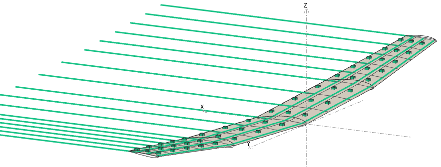
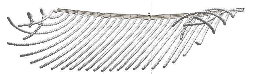
The Vortex Particle Wake
A very elegant and effective solution to many of these problems is the Vortex Particle Wake (VPW).
It's main characteristic is to describe the wake as a set of Lagrangian particles, and to include their influence as a rotational contribution to the irrotational potential flow solution.
Early numerical testing seems to show that the VPW is a robust method, which converges easily and which requires only minimal and straightforward user input.
Conclusion
The flat wake model retains its interest in the cases of simple geometries and for quick analysis of design solutions. It is also sufficient for the calculation of stability derivatives.
For other cases such as wing-body configurations, or when targeting more accurate predictions, the Vortex Particle Wake model is recommended.
Back to top