
Stability analyses
Updated November 9th, 2020
Background theory
flow5 and xflr5 implement the theory of Etkin and Reid described in "Dynamics of flight - stability and control, 3rd edition, 1996."
A summary of the theory and the definition of the variables can be found here:
Lecture AC-1 Aircraft Dynamics
Lecture AC-2 Aircraft Longitudinal Dynamics
Lecture AC-3 Aircraft Lateral Dynamics
flow5 calculates the stability derivatives using forward finite differences. In a future version, the analytical differentiation method recommended in "Flight Vehicle Aerodynamics", M. Drela 2014 may be implemented. It is expected that the method will speed up the calculations, but it should not affect significanlty the results.
Implementation
In linear stability theory, the behaviour of the airplane is calculated as a perturbation of a stable flight condition. In xflr5 and flow5, only horizontal flight is considered, so that it is required that an angle of attack exists such that the pitching moment is null, and that the flight is statically stable for this operating point.
The determination of the stability behaviour involves the following steps:
- Define a plane and its control surfaces,
- Trim the plane and the position of its CoG such that it is statically stable,
- Define a stability analysis,
- [v7.01 beta_18] Define the control parameters as a set of gains for each of the control surfaces; this option is similar to the CONTROL setting in AVL,
- Run the analysis to calculate the stability derivatives and the flight modes,
- Post-process the results.
Notes
- The option to calculate the stability behaviour as a function of inertia parameters has been deprecated and removed from version v7.01 beta_18. This choice has been made to simultaneously simplify the user interface and the underlying code.
Instead, sensitivity analyses should be performed with T6 control polars. - Up to v7.01 beta_18 flow5 offers the option to calculate the stability behaviour as a function of the positions of the control surfaces. This option however is complicated and confusing, so that it may be deprecated in a future version. Its use is therefore not recommended.
Back to main table of contents
Step by step
Step 1: Plane geometry
Define the Plane
The project files used for this tutorial and the corresponding AVL package can be downloaded here
As in previous versions of flow5 and xflr5, define the plane geometry and its inertia such that
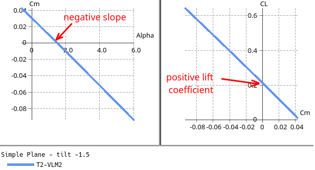
- the slope of the curve Cm = f(alpha) is negative → static stability
- the lift coefficient is positive for the aoa such that Cm = 0 → the plane flies
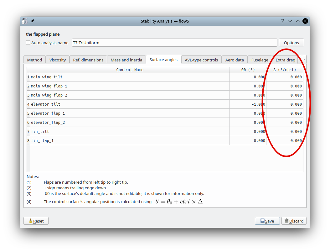
Define the control surfaces
The wing and flap angles are used as reference values for the sensitivity calculations.
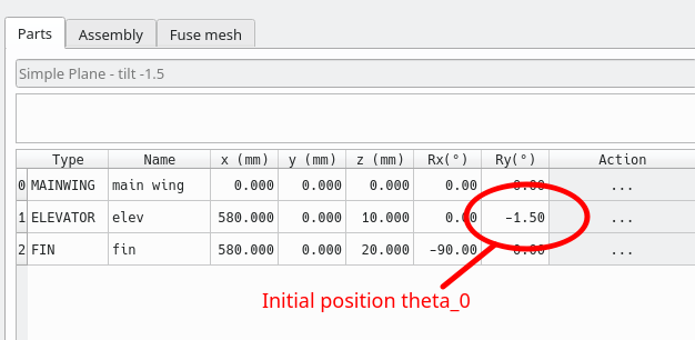
Reference angular position θ0 of each wing
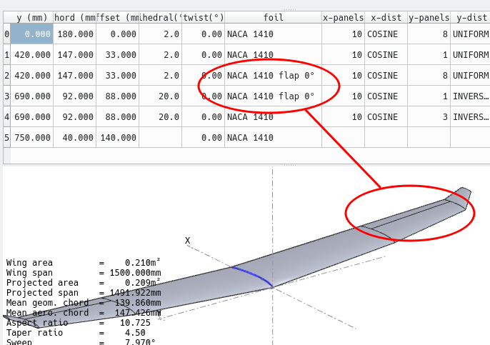
Wing flaps
The initial wing flap angle θ0 is defined by the foil flap angle.
To keep it simple, the recommendation is to set the flap angles to 0°.
Step 2: Define and run a first stability analysis
The goal is to check that the analysis gives reasonable results and that the plane is sound.
De-activate the control surfaces by setting all the coefficients to 0. As mentioned above, this feature may be deprecated and removed from a future version.
Run the analysis for any value of the control parameter: since no active control surface has been activated, the value of the control parameter is not used.
Store the operating point.
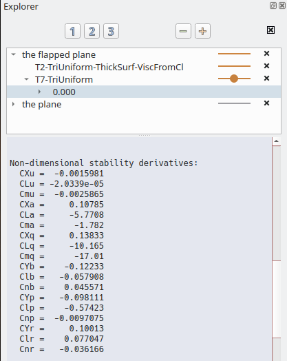
If the analysis went well, an operating point will have been generated.
Select it to access the data in the properties box, e.g. the values of the stability and control derivatives.
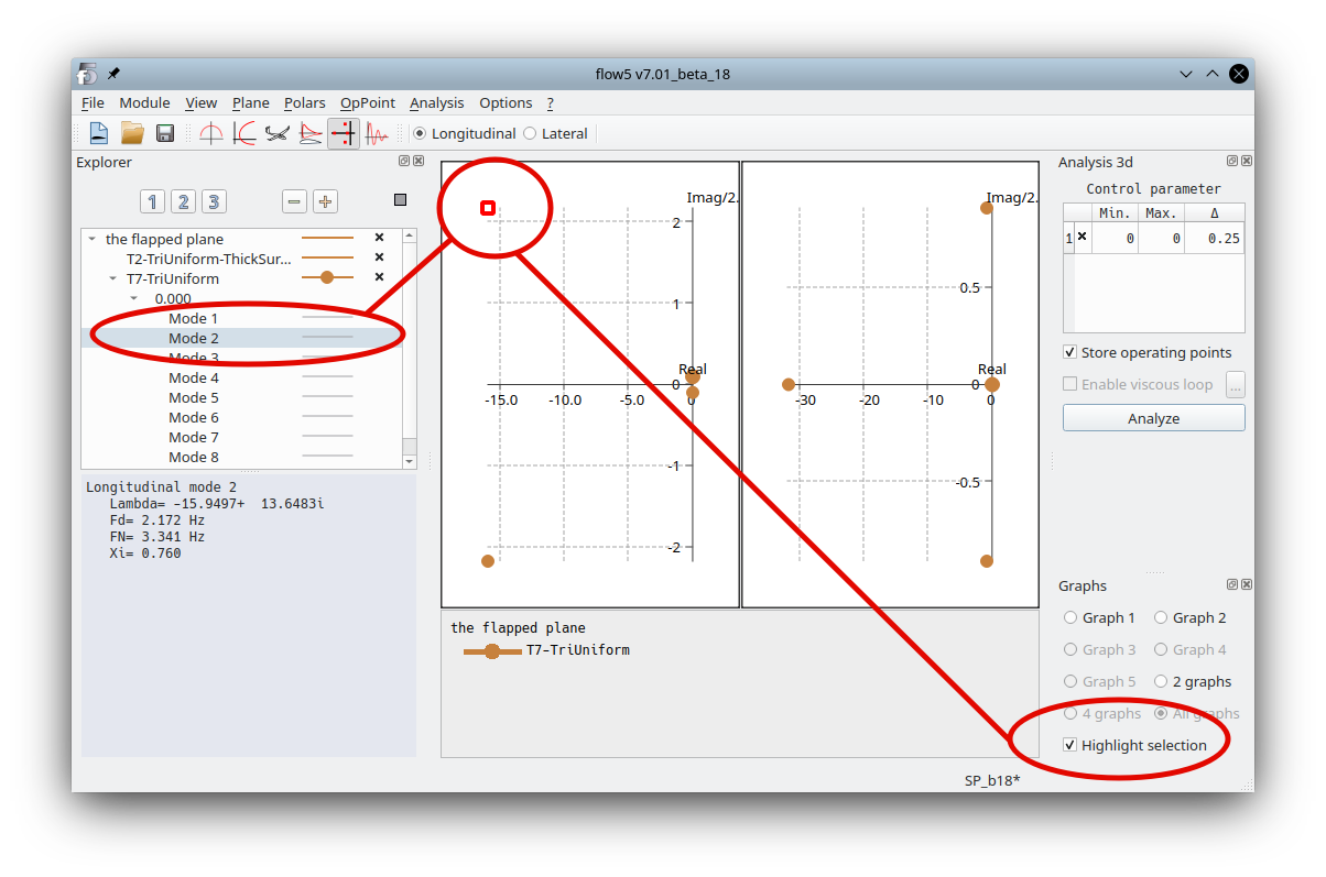
Root locus view
Check that the analysis produces the familiar conventional modes.
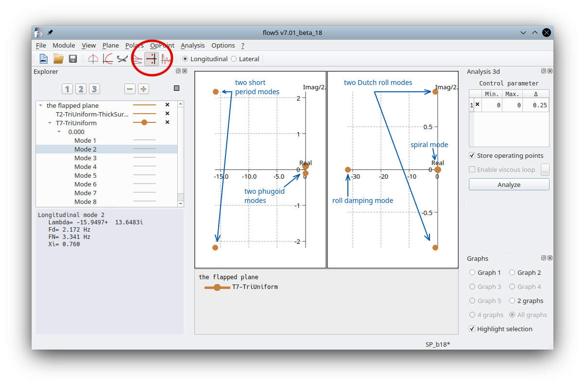
To identify a mode in the root locus graphs, select it and activate "Highlight selection" in the graph's context menu or in the toolbox in the bottom right.
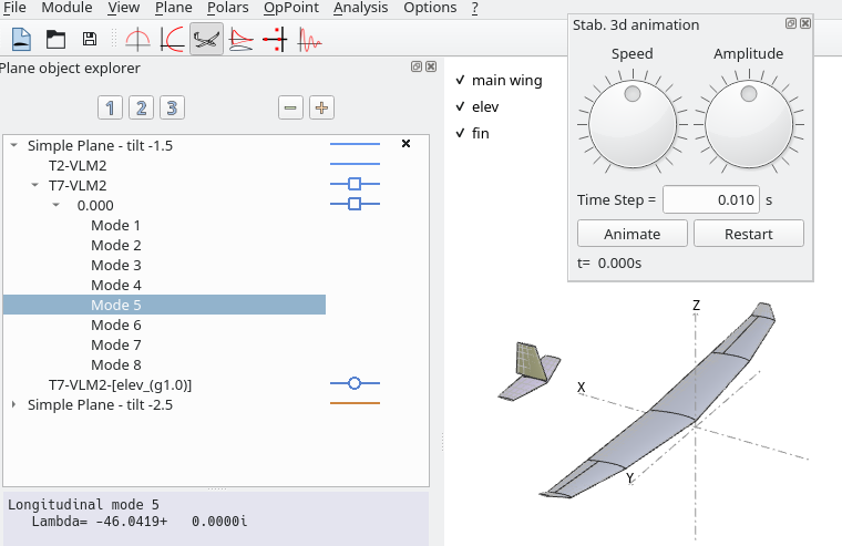
3d view
Select a mode and animate the view
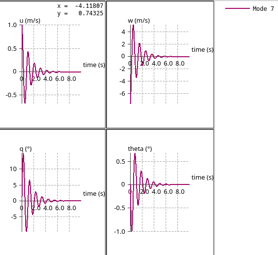
Time graphs view
Note: This post-processing module may not be as mature as the others – feedback and suggestions are welcome.
In the top toolbar, select the direction of interest - longitudinal or lateral.
Select the type 7 operating point.
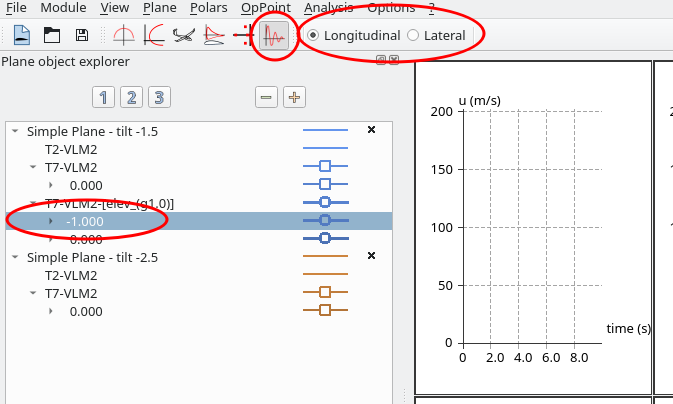
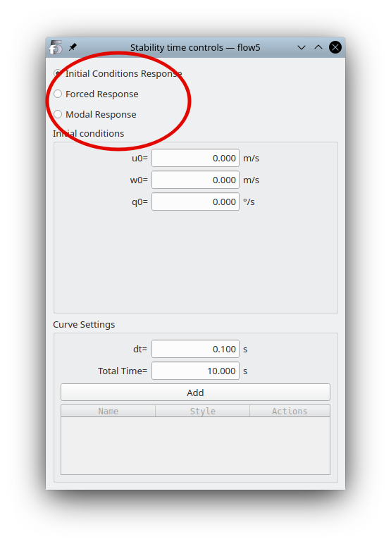
- A perturbation to the stable flight conditions
- A forced response to a control order – will be available at the next step when a control surface is defined and activated with a gain
- A pure modal response
Step 3: Define the plane's controls
The control surfaces available in flow5 are:
- the angular position of each wing around the y-axis
- the flaps defined in each wing around their hinge vector
To define a control for the plane:
- in the Stability analysis editor, move to the AVL-type controls.
- in the left column, use the context menu to add a control
- give the control an explicit name
- in the right column, define the gains for each control surface
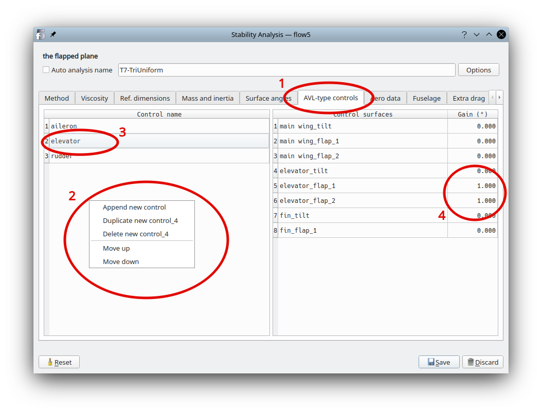
Run the analysis again. Control derivatives will be computed and output for each of non-null controls.
Response to actuation
Work in progress
Back to top