
Cp coefficients in 3d analyses
Updated April 20, 2021
------------------ WORK IN PROGRESS ------------------
Description
Background
The pressure coefficient Cp associated to a normal force F acting on a panel with area S is
Cp = F/q.S
where q is the dynamic pressure.From the numerical point of view, the pressure coefficients are the result of three main calculation steps:
- Calculation of the doublet densities,
- Calculation of the surface velocities Vlocal which are the gradients of the doublet densities,
- Calculation of the pressure coefficient using a consequence of Bernouilli's equation
Cp = 1.0 - V²local/V²∞
The second step is the trickiest, since it implies the evaluation of surface derivatives on a non-planar arrangement of panels. There are many ways to carry out this evaluation, with each involving an approximation of some kind. In fact the process is more an art than a science, and each panel code seems to have its own way of doing it.
Whatever the method, the evaluation of the pressure coefficients is one of the least precise step of a panel analysis.
In the case of flow5, the method depends on the type of panel method.
Quad panel analysis
In this case the process is exactly the one described in the reference document T.N. NASA 4023. It is the method implemented in xflr5. Please refer to the report for detailed explanations.
Galerkin triangle method with uniform doublet densities
Panel neighbours
The task at hand in this case is to evaluate a surface gradient of a scalar quantity, i.e. the doublet density, uniform on each panel and on each of its neighbours. Each triangular panel may have between 1 and 3 neighbours, and the method is adapted to each case.
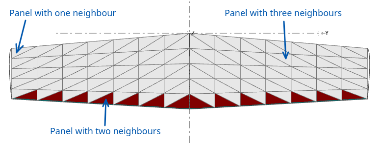
Triangle with one neighbour
In this case the gradient is in the direction of the line passing through the two triangles' CoG, and it is evaluated by first order finite difference.
Triangle with two or three neighbours
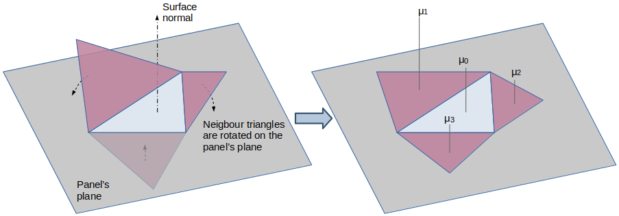
In this case, the method used in flow5 is to
- develop the panel's neighbours in the panel's plane by rotation around the edges,
- use a least square method to find the plane approximating the doublet densities μi located at the panels' CoG,
- take the gradient of this plane to obtain the local velocities.
In this case the regression is an exact solution unless the three COGs are aligned, in which case the regression is not possible. In addition, the regression becomes imprecise if the CoGs are nearly aligned.
In such cases, flow5 evaluates the gradient by second order finite difference along the average line passing through the three CoGs.
Notes
There are several problems associated with this method.-
Because the evaluation methods differ depending on the number and arrangement of neighbours, local discontinuities of the Cp colour map may be artificially created and displayed. This occurs typically at the edges and corners of a wing's surface.
A solution could be to extend the number of panels taken into account in the case of a triangle with a single neighbour by including the neighbours' neighbours. However the pressure coefficients at wing tips and edges are likely to be evaluated incorrectly anyway due to the tip vortices, to the trailing edge shear and to the inviscid assumption. Trying to improve the method further does not seem worthwile. - At locations of sharp geometrical changes such as the junction of fuselage and wing, the development of the panels on a plane may be too coarse an approximation. However these locations are likely to be turbulent and the result of a panel analysis are likely to be imprecise at this location, so that results will need to be considered with caution whatever the evaluation method.
Galerkin triangle method with linear doublet densities
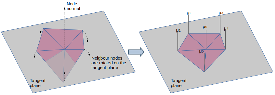
In this type of analysis, the doublet densities are evaluated at the mesh's nodes instead of at the triangles CoG.
The evaluation method of the pressure coefficient at each node depends on the number of neighbour nodes, which can range from two to any number.
The process is similar to the one followed in the uniform case:
- The neigbour nodes are developed on a plane defined by the node's position and the surface normal at this node
- The gradient is evaluated by linear regression of the μi at the developed nodes location.
Notes
This method has the advantage of simplicity but it suffers from drawbacks similar to the ones mentioned in the case of the uniform method.
Mainly, it is likely to be imprecise in the case of strong local surface curvatures or at sharp geometrical locations such as the junctions of wing and fuselage.
Wing pressure coefficients
Cp plots
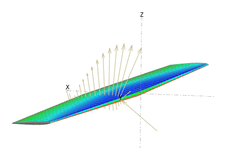
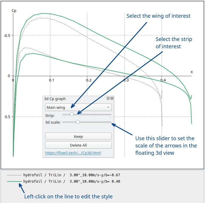
The pressure coefficients can be plotted in flow5 along the wing's streamwise strips. The Cp profile can be viewed simultaneously in the Cp graph (F9) and in the floating 3d window (Ctrl+Shift+V).
Quad panels
The Cp values are taken at the panel's centroid.
The quad CoGs are aligned by default in the streamwise direction, unless the strip is distorted by the presence of a fuselage.

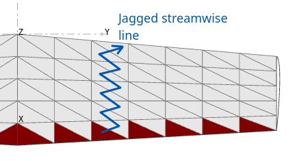
Triangular panels - uniform densities
The Cp values are taken at the panel's CoG.
Since the panels CoG along a streamwise strip are not aligned, the Cp curve exhibits a jagged shape.
Also note that the trailing edge panels have only two neighbours, and that the CoGs are nearly aligned. This makes the evaluation of the Cp coefficient difficult for the reasons explained above, and creates the small discontinuities which can be viewed at the curve's TE point.
The triangular uniform method is therefore not the preferred method for the evaluation of pressure coefficients.

Triangular panels - linear densities
The Cp values are taken at the panel's node.
The nodes are aligned by default in the streamwise direction, unless the strip is distorted by the presence of a fuselage.
The linear method offers the advantage of a higher order representation which is useful in the area of the leading edge where the pressure gradient is strong.

Validation
https://flow5.tech/data/project_files/AR_study.fl5
Influence of the panel method
The pressure coefficients have been evaluated at the center of a rectangular wing with aspect ratio = 20 and compared to XFoil results at Re=400K.
The wing was meshed with 11 quad panels in the streamwise direction with a COSINE type distribution.
The results show close correlation with XFoil's prediction despite the low number of streamwise panels.

Leading edge
A second calculation has beeen carried out with a mesh density increased to 23 panels in the streamwise direction, to improve the precision of the predictions in the LE area. The correlation with XFoil remains good.
The deviation at the trailing edge may be due to the viscous effects which are taken into account in XFoil and not in flow5.

Back to top
Conclusions and recommendations
- For its higher accuracy, the linear triangular method should be preferred for the evaluation of pressure coefficients.
- A fine mesh in the streamwise direction is not necessary.
- COSINE panel distributions in the streamwise direction should be preferred for the higher precision in the area of the LE.
Step by step
Make sure that an operating point is activated.
Switch to the Cp view by pressing the F9 key. The controls will show up by default in the bottom right area.
Select the wing of interest in the control window's top list box
Use the slider underneath to select the spanwise strip of interest.
Optional: open the floating 3d view (Ctrl+Shift+V) to view simultaneauously the Cp coefficients in 3d. Use the slider marked "3d scale" to set the length of the arrows.
Once the section of interest is reached, click the "Keep" button.
Repeat the process for other strips, other wings, other operating points or other planes. There is no limit to the number of curves which can be added to the graph.
Use the context menu in the graph to add external curves from other sources.
To edit a curve's style, click on the line button in the legend.
Back to top