Linear combinations
Updated May 19, 2021------------------ WORK IN PROGRESS ------------------
Purpose
flow5 v7.13 introduces an option to generate once unit solutions to the panel problem and to reuse them to generate results across all type 1, 2, 3, 5, 7 and 8 analyses for a given plane and mesh configuration.
The goal of the option is to take advantage of the linear properties of the panel problem to reduce the computation times.
To illustrate the benefit, once a T1 or T2 analysis has been run
- a change to the plane's inertia properties will not modify the mesh, so that a new analysis run will reuse the linear solution instead of constructing and solving the linear system again
- a T7 analysis will also reuse the linear solution
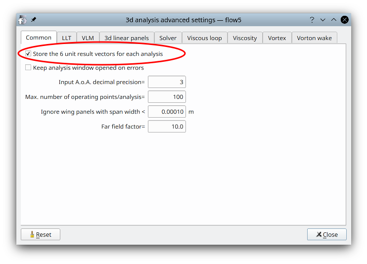
The option is activated by default and does not require any user action. It can be deactivated in the analysis settings.
This simplification has been an opportunity to introduce the more versatile type 8 analyses.
Description
Linear system
The solution to a panel analysis comes down to the resolution of a linear system with equal number of variables and equations. The different steps leading to the construction of the linear system are described for instance in the Technical Note NASA 4023.
The most computationally expensive tasks in the process are
- the construction of the influence matrix,
- the construction of the RHS vectors,
- the LU-factorization of the influence matrix
On the other hand,
- once the influence matrix has been factorized, and elementary solutions have been generated, the assembly of any general solution by linear combination is fast
- the size of the matrix prevents it from being stored durably in live memory, but there is no such issue with the storage of the elementary (unit) solution vectors
These observations form the basis of the solution method by linear combination of unit results.
System matrix
It is referred to as the "influence" matrix since item aij contains the influence of a unit doublet density distributed on panel j at the location of panel i. It is a dense matrix, since each mesh panel has an influence on all the others. For comparison a finite element matrix is sparse, since a mesh element is only connected to its neighbours. This is the reason why finite element meshes use considerably less memory and may have larger sizes than boundary element meshes.
The influence matrix is constructed using only the information of the surface and wake meshes. As a consequence,
- it is independent of the flow field
- it is identical for all linear analyses which rely on the same surface and wake meshes
Right hand side
The right hand side vector (RHS) is constructed using the information of the surface and wake meshes and of the fluid's velocity field. The important point is that the information specific to each analysis ends up in the RHS of the linear system and not in the influence matrix.
In the typical case of a solid body movement such as the motion of a plane in a static atmosphere, each analysis defines a velocity field. This velocity field is usually specified by the angle of attack α, the sideslip angle β and the speed V∞. It can also include a rotational part which is typically of use in the estimation of the stability derivatives.
In all cases, this velocity field is a linear combination of the 6 unit velocity fields defined by elementary movements along the 6 degrees of freedom in motion, i.e.
- three solid body translations along the x, y and z axes,
- three solid body rotations about the x, y and z axes
Linear combinations
Since type 1, 2, 3, 5, 7 and 8 analyses all use the same arrangement of surface and wake panels and therefore the same influence matrix, it makes sense to calculate once the unit elementary solutions and to store them for future use by these analyses. Once the unit solutions are available, the LU-factorized influence matrix is discarded.
Type 1, 2, 3, 5, 7 and 8 analyses are referred to as "linear analyses" herafter.
On the other hand in the case of type 6 analyses, the wake panels or particles depend on the velocity field. This implies that the influence matrix depends on the velocity field, and that the linear system needs to be built and solved for each operating point.
Default method in v7.13
The generation of results by linear combinations is the standard procedure used by panel codes such as XFoil and AVL. It is also the method used in flow5 to calculate all the operating points in an analysis run.
The main change in v7.13 is that the unit solutions are kept in live memory instead of being discarded at the end of the run. This saves steps (1) to (3) of the linear system resolution for subsequent calculations of polars and operating points.
Whenever a linear analysis is requested, the application first checks whether the elementary solutions exist, and re-uses them if they do. If not, the problem is solved for the unit solutions which are then stored for future re-use.
Limitations
-
It is implicitely assumed that all the linear analyses defined for a given plane use the same settings for the wake panels. The application does not make this verification and assumes that the wake is the same in each case.
It is therefore a recommended practice to define the flat wake once and leave the parameters unchanged for all subsequent analyses. A typical setting is- 5 wake panels in the streamwise direction
- a wake length equal to 100 MAC
- a progression factor equal to 1.1
- The unit results are cleared each time that the mesh becomes invalid, e.g. when the plane's geometry or mesh is modified, or when the wake settings are modified.
- The unit results are valid for one type of analysis and one type of surface mesh. A VLM, a quad analysis, a tri-uniform analysis and a tri-linear analysis will each require their set of unit solutions. Thin and thick surface analyses will also each require their set of unit solutions. It can therefore be a good practice to use the same type of analysis throughout the project.
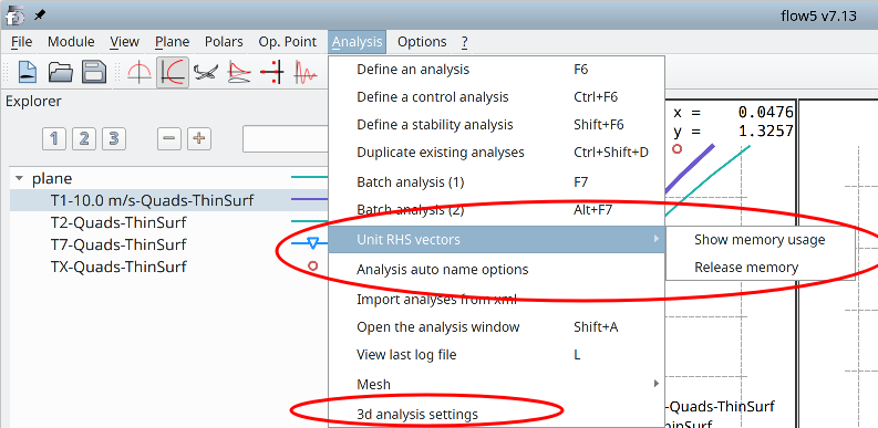
- The storage of the unit solutions requires minor additional memory usage. This memory space is typically negligible compared to the space occupied by the influence matrix. It can become significant in extreme cases where a high number of analyses of different types are carried out for a high number of meshes. The space occupied can be checked and released at any time using the option in the top menu "Analysis/Unit RHS vectors".
-
The control derivatives cannot be evaluated using linear combinations of the unit results since the mesh and therefore the influence matrix are modified by the rotation of the control surfaces. If control derivatives are requested as part of a type 7 analysis, the linear system will be built and solved to make the LU-factorized matrix available for the calculation of the derivatives.
Note for the sake of completeness: the derivatives could be evaluated by linearizing the boundary conditions which end up in the RHS vectors of the linear system, and by ignoring the change to the influence matrix. This is how panel codes usually evaluate the derivatives, and experiments in flow5 show that the error when using this simplification is only a few percent.
The show stopper which prevents the activation of this option is that it would require that the factorized influence matrix be stored in live memory for each pair of plane and analysis, which is not achievable.
Back to top
Validation
It has been checked that the analysis results are the same whether the option is activated or not.
This verification can be performed at any time by activating and deactivating the option.
Back to top
Step by step
The option is activated in the interface of the analysis settings. This interface is accessed in the top menu "Analysis/3d analysis settings".
The menu option "Unit RHS vectors" enables the control of the live memory used by the RHS vectors.